
Mar 13, 2021
Many games that feature procedurally generated worlds divide the worlds into individual biomes. The biomes often have separate terrain or features, which need to be blended smoothly at the borders. Most of the common or intuitive solutions suffer one of two shortcomings: they’re slow, or they have visible grid patterns. In this post, I will demonstrate a method which avoids the latter with a much better tradeoff in the former. The method involves two main components: Voronoi-noise-style data point distribution, and normalized sparse convolution.
Defining the Output
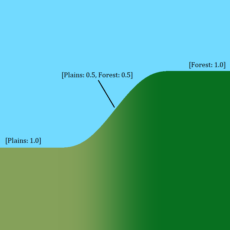
To implement effective biome blending, there is certain data I want to produce at each point in the world. To make the blending portable to a wide variety of scenarios, the idea is to produce weight values that correspond to the contribution each biome makes at a particular coordinate. For example, the blender might output weights {Forest: 0.6, Plains: 0.4} somewhere inside the transition zone between the two biomes. If our goal is to compute terrain height, then we can add together the weighted biome heights as follows: Forest.GetHeight(...) * 0.6 + Plains.GetHeight(...) * 0.4. It would also be possible for three (or more) biomes to merge near a corner: {Forest: 0.55, Plains: 0.24, Mountains: 0.21}, or to be entirely inside one biome: {Plains: 1.0}.
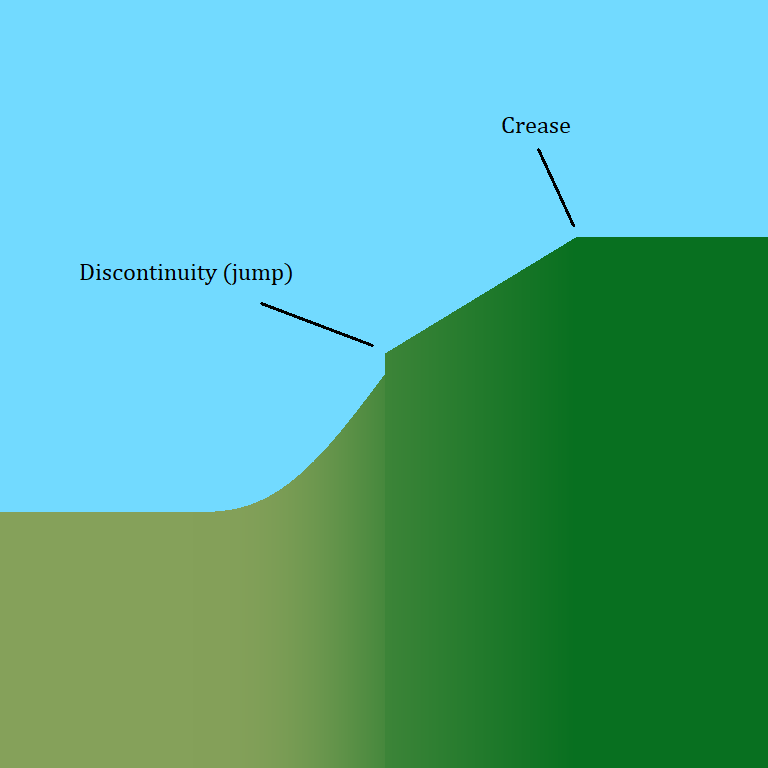
Importantly, these weights should change gradually throughout the world, so that they do not introduce any jumps (or creases either ideally) into the world generation. This way every border is a smooth ramp between the values each biome would produce on their own. The weights should also always add up to one at a given coordinate. For a location entirely inside one biome, a weight of one means the biome can decide the terrain features without any unintended rescaling. Where biomes mix, this makes sure the ramp doesn’t form a bump or a dip if the blended values are extreme.

There are many ways to arrange the data, all of which provide the same information. I will cover the format I used later in the article.
Methods and Problems
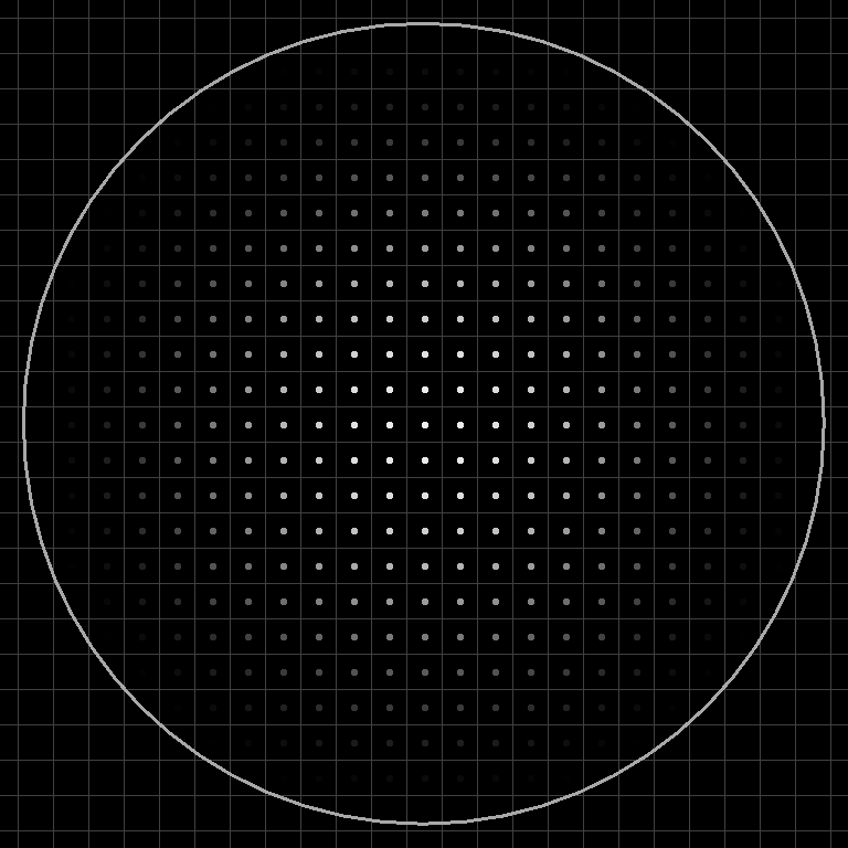
A simple blending algorithm might consist of generating the biome map in full resolution, then performing a Gaussian-like blur on it to produce the blending weights. To do this, you might start by populating the map in a large enough area around the part of the world to be generated. If your world is generated in sections or “chunks”, then you might employ caching here to prevent repeatedly generating the same areas. After this, consider a circle around each column or pixel coordinate to generate the terrain for. On the biome map, set up like you’re going to count the number of cells of each biome that show up inside the circle. But instead of adding one each time, add a number that decreases with distance. I might use the formula max(0, radius^2 - dx^2 - dy^2)^2 for this. It produces a circular bump like a Gaussian filter, but it goes zero smoothly at a finite radius. To make the biome weights add up to one, each needs to be multiplied by the reciprocal of the total. Because the total is constant, the reciprocal can be precomputed.
Update 03/31/2021: A handful of readers were astute to point out that a Gaussian filter is separable. This means the blurring operation can be performed using two fast steps along each axis, instead of one slow step over the full range. I have removed the wording that described the polynomial as faster. While this is true when comparing individual formula point evaluations, it can cause confusion due to the different opportunities for optimization that each option presents in this case. It also becomes inconsequential if the filter is pre-computed and stored in an array.
If the biome generation is fast, then the full-resolution blur works ok for small blending circle sizes. But as the radius increases, the loops over every coordinate start to take large amounts of time. And, if the biome generation itself isn’t fast, then calculating it for every coordinate can cause its own performance problems. I implemented this a while back, and was not always satisfied with its speed.
Some generators skirt around this by generating everything on a lower resolution grid, then interpolating between the gaps. This addresses the speed problem, but it prevents the borders from producing any angular variety below the scale of the grid. It pulls the borders into alignment with the grid edges, because the only data available is at the corners. It also creates regularly-spaced creases when only basic linear interpolation (lerp) is used. These issues become particularly apparent when the borders try to take on details that the grid is too coarse to capture. Minecraft is a notable example which uses this strategy, and someday I plan to write a series of articles where I suggest and implement improvements to many of the techniques Minecraft uses. For now, I will cover biome blending on its own, in a manner not specific to any game.
Solving Both Problems
The interpolated grid improves performance by reducing the number of points on the biome map that need to be calculated, as well as how many the blending loop needs to consider. Its visual problems come mainly from the grid itself. If we can do away with the grid structure, but preserve efficiency, then we can solve both problems.
In my solution, I replace the grid with randomly distributed data points. Then, I blend over the points using normalized sparse convolution.
Distributing Points
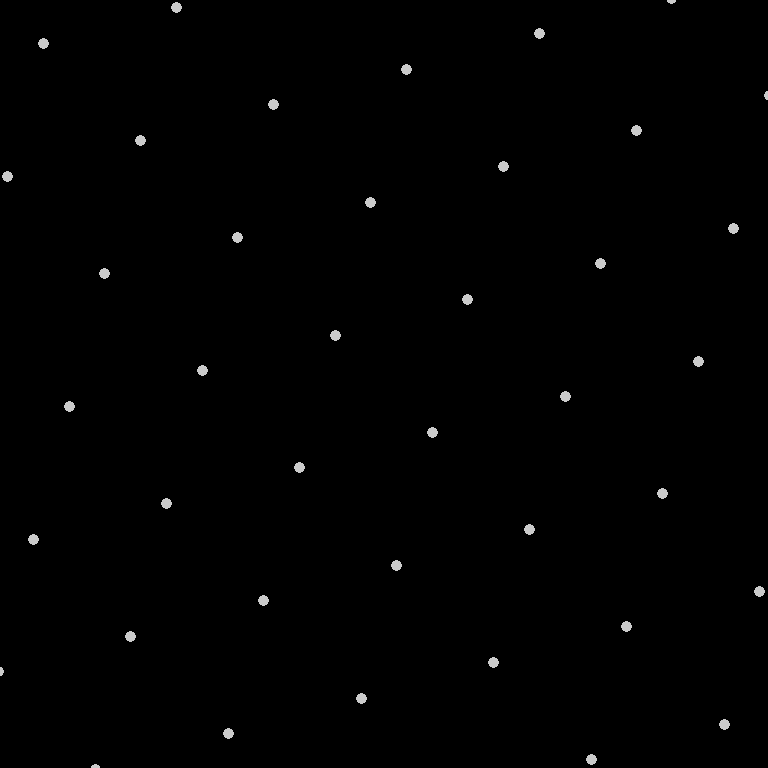
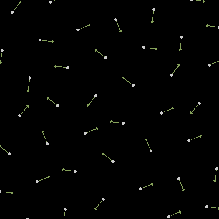
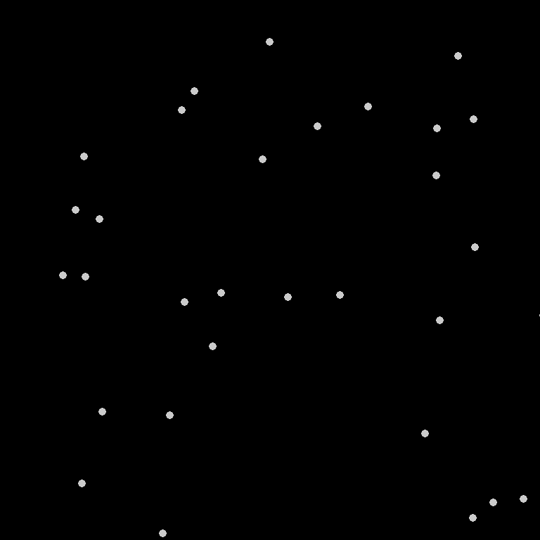
To produce the point distribution, I used a jittered triangular/hexagonal grid. Each vertex on the grid is displaced in a randomized direction by a fixed distance, similar to how Voronoi noise is often implemented. This creates a distribution that appears random, but doesn’t have any large gaps. A jittered square grid can also work, as is shown on the linked page at RedBlobGames. However, the triangular option confers less possibility for visible axis alignment. For this reason, I consider the triangular basis to be a better choice for most terrain generation applications. Blue Noise point distributions would be even better – in particular you can use Poisson disc sampling if your world is finite and small. I might explore this more in a future article. This RedBlobGames page demonstrates and compares all three of these distribution types.
Because a jittered grid is able to avoid large gaps, it is possible to choose a base size for the blending circle, so that it will always contain or intersect points. From there, padding can be added to ensure there are no unreliable edge cases, as well as establish a minimum width for border transitions.
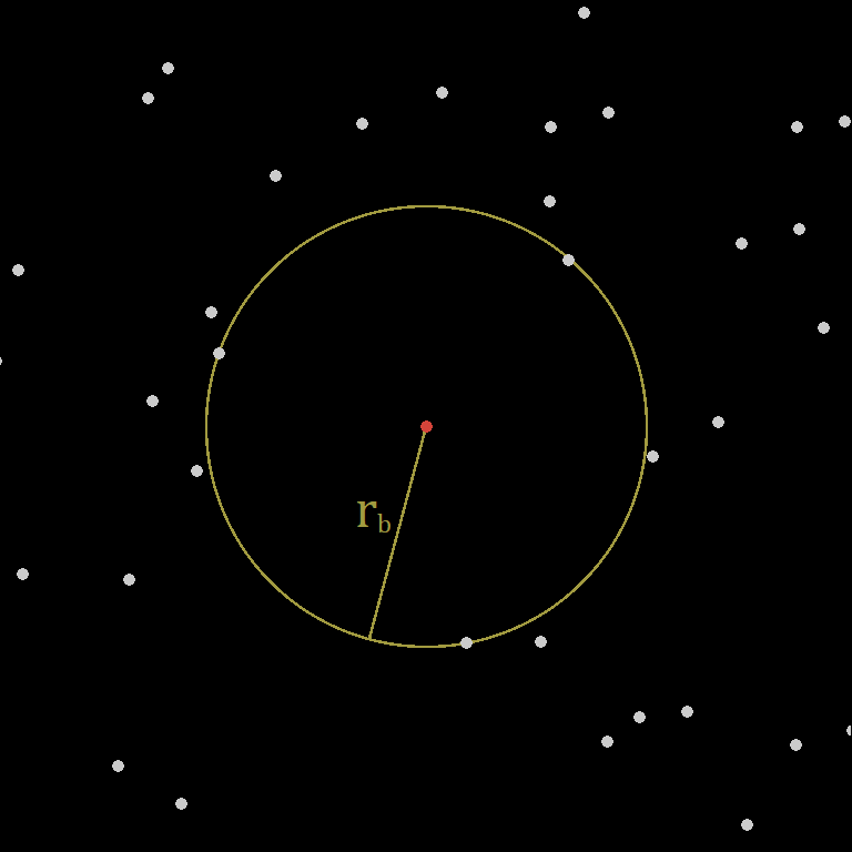
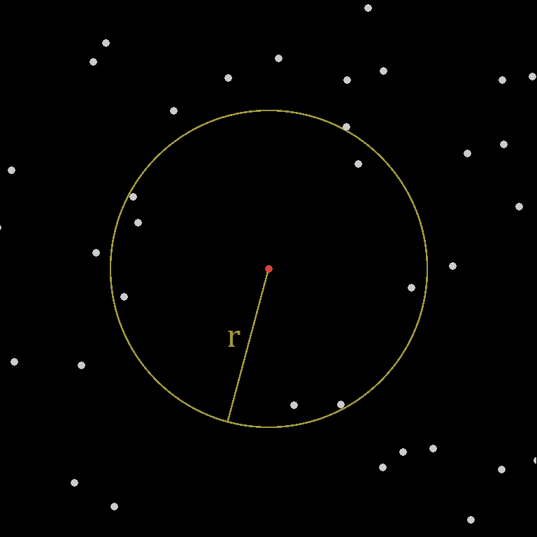
Finding Points
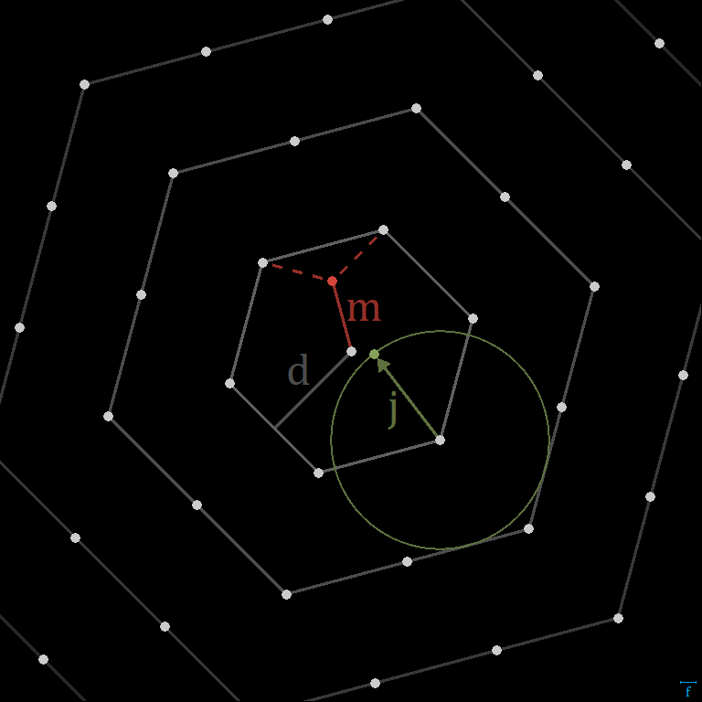
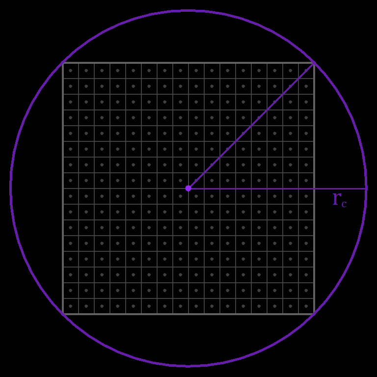
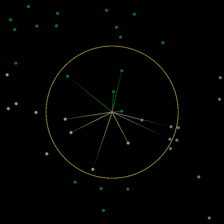
If we know the size of the blending circle we will use, then we can determine how far out to search the grid for data points. Since we’re no longer using a coordinate-space-aligned grid (unless your world is also triangle/hex based), we can’t just scale and offset to determine a grid range. We can, however, still enumerate all of the points we need. If we locate the closest vertex on the unjittered grid, then we can iterate outward in hexagonal layers until we know we’ve looked far enough.

With this in mind, it is possible to perform the search only once per world-chunk. In this case, choose the center of the chunk as the starting point. Then, find the radius of a circle containing the chunk, and add it to the total search range. An important characteristic of this approach, is that it lets us query all of the points needed for a chunk, but they are not defined per chunk. This way, chunks can do their job of hosting the world and streamlining generation, without making any undue contributions to its shape. Using the maximum distance to the closest grid vertex, jitter magnitude, frequency, effective chunk radius, and distance per layer, we can calculate a reasonable upper bound on the number of layers to search. Then, we can precompute the actual list of relative points to process each time. During generation, the base vertex and jitter are added to the relative point coordinates in the list, and any points out of range are culled.
Normalized Sparse Convolution
Each jittered point samples the biome map at its location. To generate blending from this data, the process is similar to the Gaussian-like blur described previously. First, a formula determines a weight that each data point should contribute to its respective biome. Here, I continue to use max(0, radius^2 - dx^2 - dy^2)^2. However, because the new points are distributed few and far between, the total weight per coordinate becomes wildly inconsistent. To correct for this, it is necessary to compute the total and its reciprocal dynamically, before multiplying the weights by it. Once this normalization step is in place, the output meets the sum requirement again.

The Results
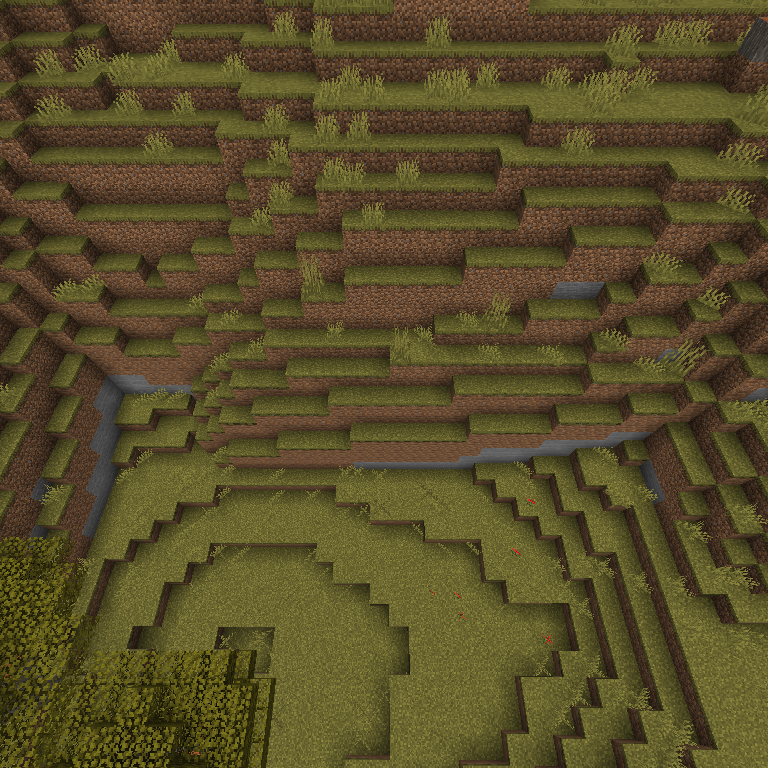
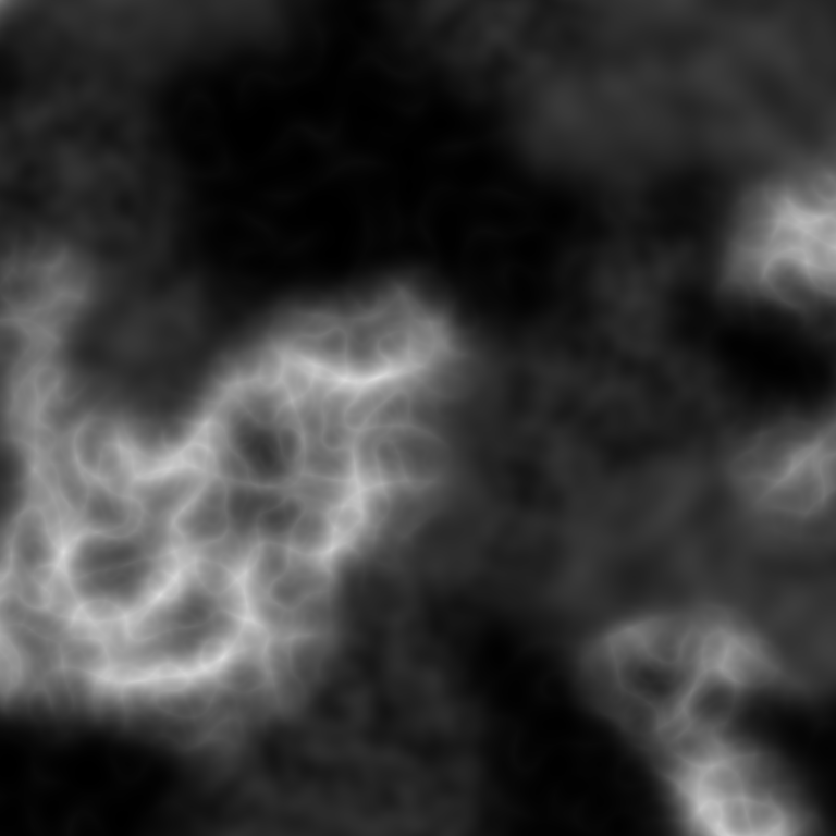
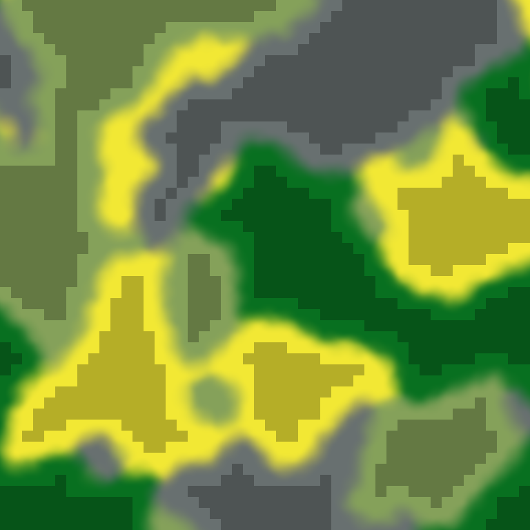
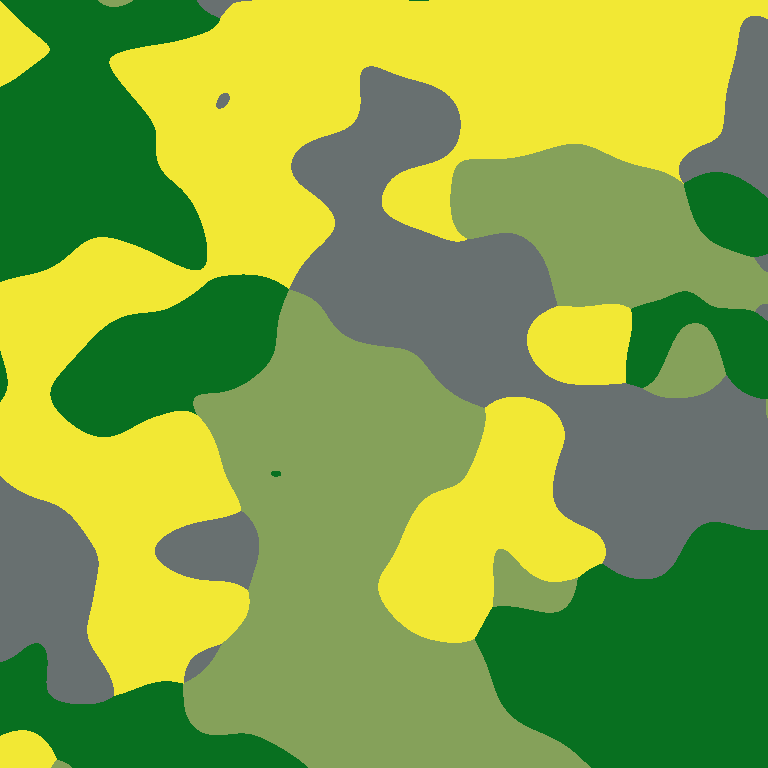
To demonstrate this algorithm, I created a simple utility that displays each blended biome as a unique color. To give it something to work with, I needed a callback function. Biome generation itself is an involved topic worthy of its own article, so I created a basic one for this. It generates one instance of OpenSimplex2S fractal noise per biome, then chooses the one with the highest value.
Here are some results produced with it. I generated four images to show two different sampling frequencies, as well as two different radius padding values.


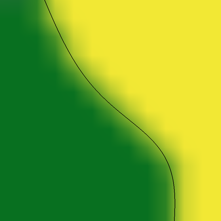
The blending appears to work nicely, contributing no visible grid patterns to its final result. What is present, is a noisy effect on the borders, consisting of fluctuations in both position and width. This may be a desirable effect in some scenarios, and may even serve as a substitute to domain warping. However, it can be controlled if necessary. Increasing the point sampling frequency reduces the warping, and increasing the radius padding covers it up with wider transitions.
Comparison
To see how this stacks up against other approaches, I created some mockup implementations. Here, I compare the scattered blend to the full-resolution blend, the lerped grid blend, and a bonus grid-based sparse convolution. Because the scattered blend accepts a radius padding rather than the full radius, I chose the padding so as to achieve the same internal blend radius. I also chose its frequency so as to produce the same average number of sampling points in a given area. In a real scenario, a developer would probably tune this manually, rather than try to mathematically fit it to certain requirements.
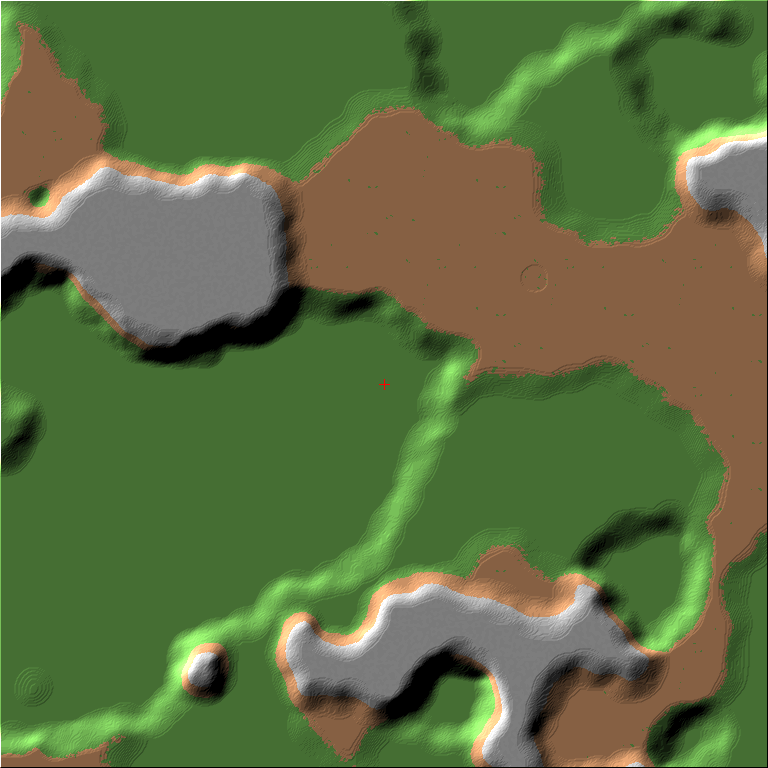
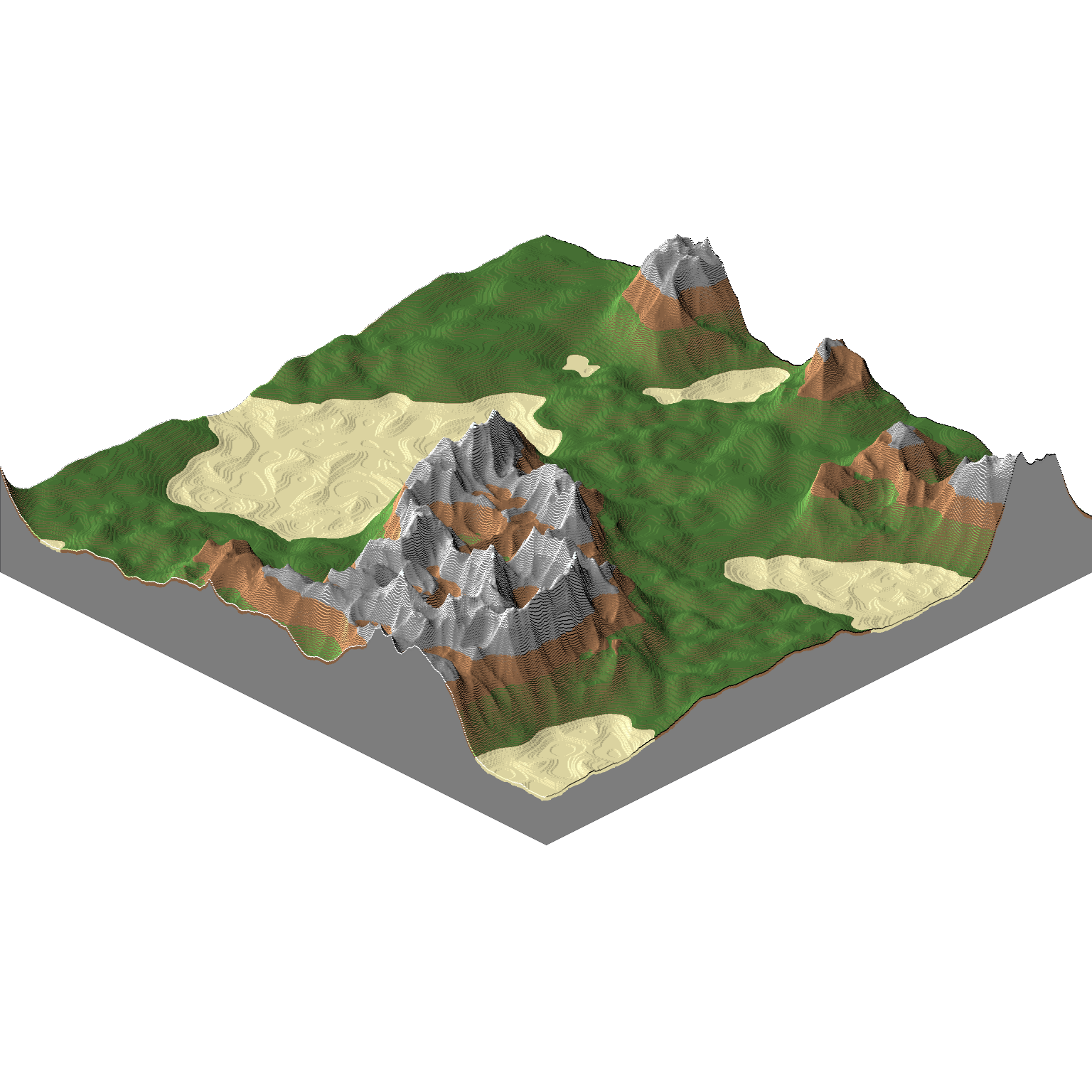
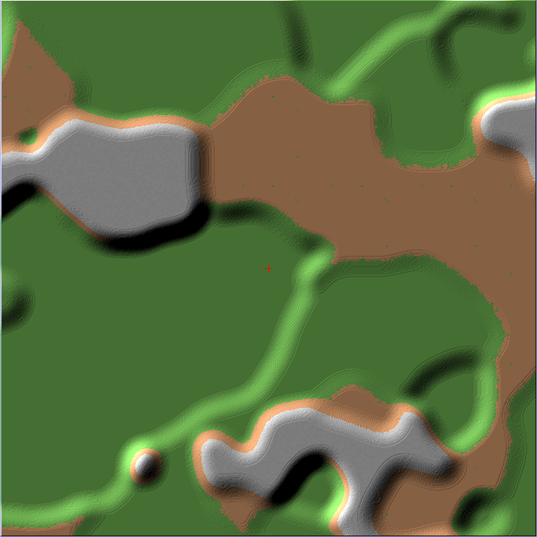
Aside from the waviness of the scattered blend, the color-blended images proved not the best medium to showcase the differences. So instead, I imported them into WorldPainter as heightmaps, which highlights the slopes. I linked to the original images in the captions.


As expected, the simple (full resolution) blend produces the smoothest results. The scattered blend adds an inherent noisy aspect to the borders, but importantly it does not introduce any apparent angular bias. The lerped grid has by far the most visible grid patterns. The convoluted grid blending produces smooth results, but the curves are pulled to follow the grid.
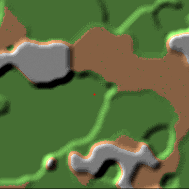
To see if I could get better results from the grid cases, I doubled the grid frequency and left the radius the same.


The interpolation intervals on the denser lerped grid are less visible from an aerial view like this. However, they are still the most visible of the axis-biased artifacts, consisting of regularly-spaced creases in the terrain. Particularly, they remain quite apparent at the local scale of the world that a first-person player would experience. If the linear interpolation itself were performed on a jittered triangular mesh, then I would find the creases less problematic. It is the grid nature of the creases that leads me to reject this approach.
In the denser convoluted grid, there are no creases, and there is much better preservation of directions. However, there is still some of a square grid effect, whereas the purpose of this article is to avoid it entirely. Many of the borders that are already running roughly 45 or 90 degrees, seem to lie parallel enough to the grid’s sampling points that it pulls them completely into following those angles. Some of the transitions also repeat shapes based on the grid, which can become apparent when blending between large height differences. Regardless, it is vitally dependent on its parameters to produce decent results, which can lead to problems in user-customizable worlds. With these parameters, though, it’s better than it was previously, and a bit of jitter might solve the remaining issues.
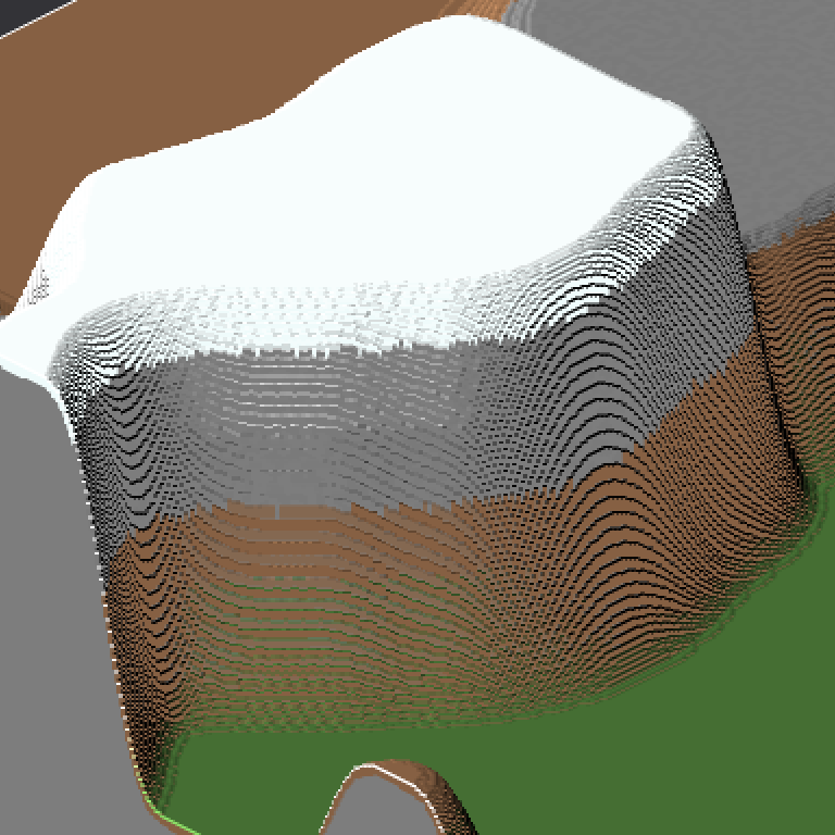
Heightmap Example
Rendering the blended colors can be useful on its own, but it doesn’t show us how this would actually look in real terrain. Here, I assign each biome its own heightmap formula using OpenSimplex2S noise, and blend between them using the scattered biome blender.

Performance
As discussed at the beginning of the article, efficiency plays an important role in making this approach viable. More specifically, it should present a better tradeoff between quality and performance compared to either the interpolated or full-resolution case. I ran some tests to measure its performance compared to the other methods, as well as how the parameters affect it. Here are the initial results, in nanoseconds per generated coordinate on my machine. Lower is faster. Note that I implemented a caching step in the scattered blending’s biome map evaluation to compensate for the full-map pre-generation advantage I gave to the other three cases.
| Full-Resolution | Scattered | Convoluted Grid | Lerped Grid | |
|---|---|---|---|---|
| gi=8, r=24 | 6818.692 | 305.745 | 148.508 | 23.895 |
| gi=4, r=24 | ’’ | 1114.819 | 463.857 | 89.579 |
| gi=8, r=48 | 25049.832 | 763.721 | 442.121 | 40.518 |
| gi=4, r=48 | ’’ | 2904.640 | 1624.995 | 220.749 |
This already shows clear differences between the runtimes of each case. However, there is a straightforward optimization that lets us do better.
An Optimization
In a typical use case, many nearby points will sample the same biome. It is only as the borders approach, that points belonging to different biomes will show up inside the blending circle at the same time. Because of this, it is possible for an entire chunk to be covered by only one biome. In fact, for sufficiently large biomes, this will be the most common case. If we check for this, then we can skip the blending entirely in these parts.
Here are the updated performance metrics. In the interest of fairness, I added the optimization to all four cases.
| Full-Resolution | Scattered | Convoluted Grid | Lerped Grid | |
|---|---|---|---|---|
| gi=8, r=24 | 4851.143 | 195.662 | 97.646 | 21.511 |
| gi=4, r=24 | ’’ | 805.298 | 329.614 | 77.301 |
| gi=8, r=48 | 23136.046 | 664.923 | 397.046 | 40.174 |
| gi=4, r=48 | ’’ | 2662.248 | 1499.852 | 209.106 |
Applying this optimization increases performance by up to 36% for the scattered case. The full-resolution and convoluted grid cases follow closely (~29% and ~34% max), while the lerped grid shows the least improvement (~14% max).
For given parameter values, the scattered blend is not as fast as the convoluted or lerped grid cases. It is, however, significantly faster than the full-resolution (“simple”) blending. This difference becomes especially apparent when using lower point sampling frequencies – an option not afforded to the simple blending case.
The convoluted grid case is faster than scattered, however its grid artifacts only start to become convincingly hidden for grid intervals ≤4. At that point, you lose enough of its performance advantage that it would be easy to instead pick a lower sampling frequency for the scattered case, such that it is faster at the same time as lacking visible grid artifacts.
The linearly interpolated case is always the fastest, however its grid artifacts are so visible that the speed isn’t worth it in my view. You can try a grid interval of 2, which looks a lot better than 4, but this increases the above runtimes to 594.905 (r=24) and 2025.882 (r=48). These times are easy to beat with scattered blending.
Chunk Size
The metrics above were all generated using 16x16 chunks. Moving up to 32x32, they change as follows:
| Full-Resolution | Scattered | Convoluted Grid | Lerped Grid | |
|---|---|---|---|---|
| gi=8, r=24 | 5502.449 | 235.809 | 113.434 | 21.378 |
| gi=4, r=24 | ’’ | 989.238 | 392.225 | 73.194 |
| gi=8, r=48 | 24351.690 | 768.681 | 432.915 | 34.134 |
| gi=4, r=48 | ’’ | 2900.521 | 1594.159 | 173.820 |
Interestingly, lerp ran a bit faster, while the other cases fared slightly worse. Chunk size might be out of your control depending on the scope of your use case, but it does appear to have an effect. How much of this can be attributed to cache friendliness, point querying, memory allocation, etc. I do not know for certain.
Final Performance Note
As this generation only occurs in 2D, and you may have many other steps in your terrain’s generation (e.g. 3D noise, feature placement), it might be worth considering this in context of your generator’s performance as a whole. Unless you can improve many of its parts in a similar way, focusing on percentage improvements in individual parts can lead to a skewed picture of the total percentage speedup you would gain. The scattered blending isn’t as fast as lerp, but it’s much faster than the full-resolution case. It’s also more in line with the runtime of typical heightmap formulas that consist of multiple noise evaluations ~20-100ns each (on my machine), and already faster than you can likely expect from optimized (full-resolution) 3D noisemaps.
Noisy Borders (for better or worse)
As discussed in the results section, this approach leaves a warping effect on the borders as a result of the irregular sampling. The centers of the border transitions might not correspond accurately to what the biome generation callback returns. Some form of this shows up in each algorithm tested, but it is particularly prevalent on the scattered blending with certain parameter configurations.
The effect can add variety to the world generation, but if you rely on the unblended map for other game features then the callback itself might not be reliable enough to use there. To address this, you can simply define the true biome map using the highest weighted biome at each coordinate.


The title image of this article uses this redefined biome map as well, but with different parameters that produce straighter borders.
Generality Note
The point querying technique is being used here with the specific purpose of sampling biomes from a biome map. It works great here, but its usefulness can go far beyond this too. Many other techniques that can take advantage of queryable point distributions include:
- Structure or feature placement
- Irregular interpolation
- Mimicking erosion
- Voronoi noise itself
- Other noise involving distributed points
Further Considerations
I covered many points that may come up during use of this blending. However in the interest of keeping a semblance of brevity, there is a lot that I didn’t cover or elaborate on. I may explore some of these in the future.
- Configurable biome map generation
- Adjusting the result to respect biome altitude boundaries (e.g. land/sea at sealevel)
- Preventing biome border corners on coastlines
- Variable blend widths
- Grid interpolations other than lerp
- Fast linear interpolation on the jittered grid
- Jittered square grid appearance and performance in comparison
- Unjittered triangular grid blending
- 3D Generalization
The Code
The code is available in the following repository: KdotJPG/Scattered-Biome-Blender.
The blending is accomplished in the class ScatteredBiomeBlender. ScatteredBiomeBlender generates the entire blending for a requested chunk, and outputs it in a linked-list-style data structure. Each node denotes one particular biome, and enumerates its weights for every chunk coordinate in an array. It also contains a reference to the next element, which will be valued null to signify the end. This format grows only proportional in size to the number of biomes in range, but it also avoids constructing individual instances per coordinate.
Usage of ScatteredBiomeBlender involves maintaining an instance to be used by each chunk generation call, and iterating through the LinkedBiomeWeightMap nodes it returns. It is designed specifically to work for square chunks with square pixels/voxels, but it can be reimplemented using the same concepts for other shapes too.
The ScatteredBiomeBlender maintains an instance of a ChunkPointGatherer, which supplies it with the list of local data points to process on each chunk generation call. When the list is returned from the gatherer, the blender invokes a user-specified callback on each point. The callback returns a biome for that point’s location, which is then stored so it can be referenced many times during the blending process.
ChunkPointGatherer doesn’t handle the full point gathering process, though. I split that responsibility into two classes: UnfilteredPointGatherer and ChunkPointGatherer. UnfilteredPointGatherer performs the actual search based on a frequency and radius. Its constructor removes points that cannot be jittered into range, but its query method doesn’t do any addional filtering. ChunkPointGatherer wraps UnfilteredPointGatherer, adding the needed radius padding and culling any points out of range. This way, various wrapper classes can be written instead of ChunkPointGatherer, without incurring the cost of multiple successive culling operations.
The DemoScatteredBlend and VariousBlendsDemo classes generate the biome map images that were used in this article. VariousBlendsDemo contains the mockups of the three other blending algorithms, as well as the code to produce the performance metrics. DemoScatteredBlend allows more fine tuning of the specific parameters used by ScatteredBiomeBlender, and contains the code used to generate the heightmap example. On the side, there is DemoPointGatherer, which displays the point distribution directly. VariousBlendsDemo also has this feature.