Jan 16, 2022
Noise plays an elemental role in many genres of procedural generation. One algorithm in particular, Perlin noise, has dominated the conversational spotlight, but it suffers a critical flaw: visible axis alignment. Newer approaches exist which address this problem, but such biased noise still sees widespread use where it may not be the right choice. In this article, I will dive deep into this issue and cover two of our most practical options now.
This article comprises the first segment of a two-part separation of the original. The second can be found here.
Confusion Clear-up
First, it is important that I clarify some terminology, because there are occasional discrepancies between sources.
-
(Coherent) noise: A type of procedural generation primitive which consists of continuous (typically also smooth) randomized bumps and valleys in an N-dimensional coordinate space. Multiple layers of noise can be combined in different ways to create a wide variety of effects.
-
Perlin noise: A specific algorithm for generating such noise, which smoothly interpolates between the ramps of pseudorandomly-chosen slope directions (gradient vectors) assigned to each vertex on a square/cube grid.
-
Fractal Brownian motion: A technique in which multiple layers (“octaves”) of some noise are combined to yield a new result with richer detail. Each layer is assigned a different frequency and amplitude. It’s often abbreviated fBm or simply called fractal noise.
Most sources use these terms accordingly, regardless of what their actual content is. However, a handful use Perlin noise to refer in reality to fBm, or the combination of some algorithm with fBm.
Two additional terms I will use throughout the article are defined as follows:
- (Noise) algorithm: A scheme for generating noise which includes certain defining steps.
- (Noise) implementation: A specific embodiment of a noise algorithm in code or other media.
Perlin: A Square Noise
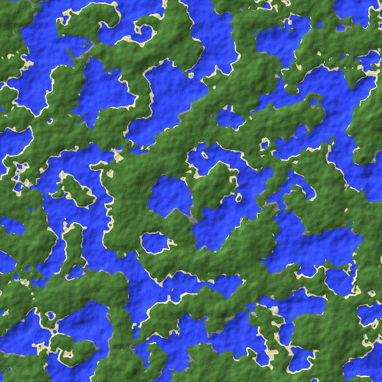
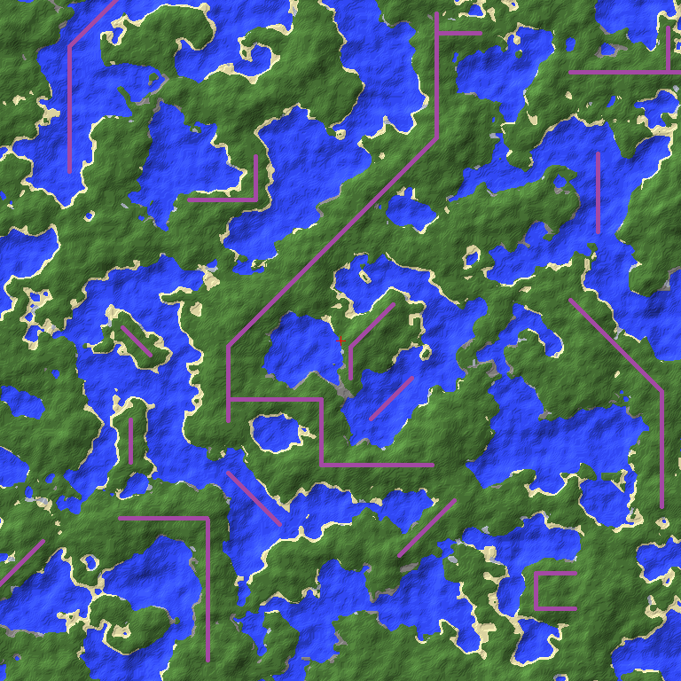
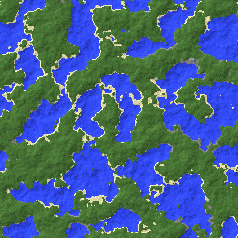
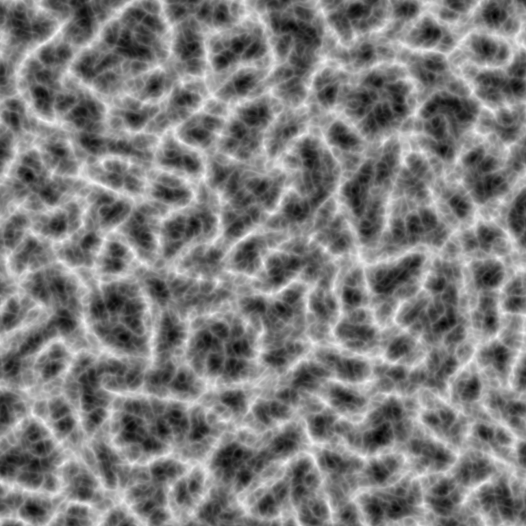
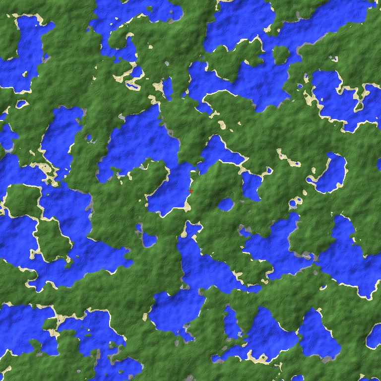
Perlin noise, so defined in the previous section, is an algorithm for generating smooth randomness. Tools like this have a myriad of applications in procedural generation, most notably in terrain generation and texture synthesis. Noise creates randomized wave patterns over multiple dimensions, which can be passed through various mathematical formulas to achieve particular results. Perlin has seen wide popularity in the noise space for quite a long time, to the point that it’s become a frequent focal point of tutorials and libraries. This noise, however, stumbles in a significant way that needs to be addressed.
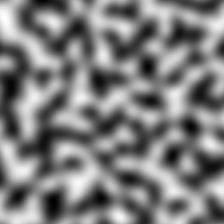
Perlin noise is visibly square-biased. It’s smooth and random, as formulas call for, but the features and shapes the noise creates fall predominantly in alignment 45 or 90 degrees to the input coordinates. This phenomenon persists globally throughout the noise, offering little break or gap in-between. Such behavior is ill-fit for applications of this category, especially if a solution is to be upheld as a standard.
Why Avoid Squareness?
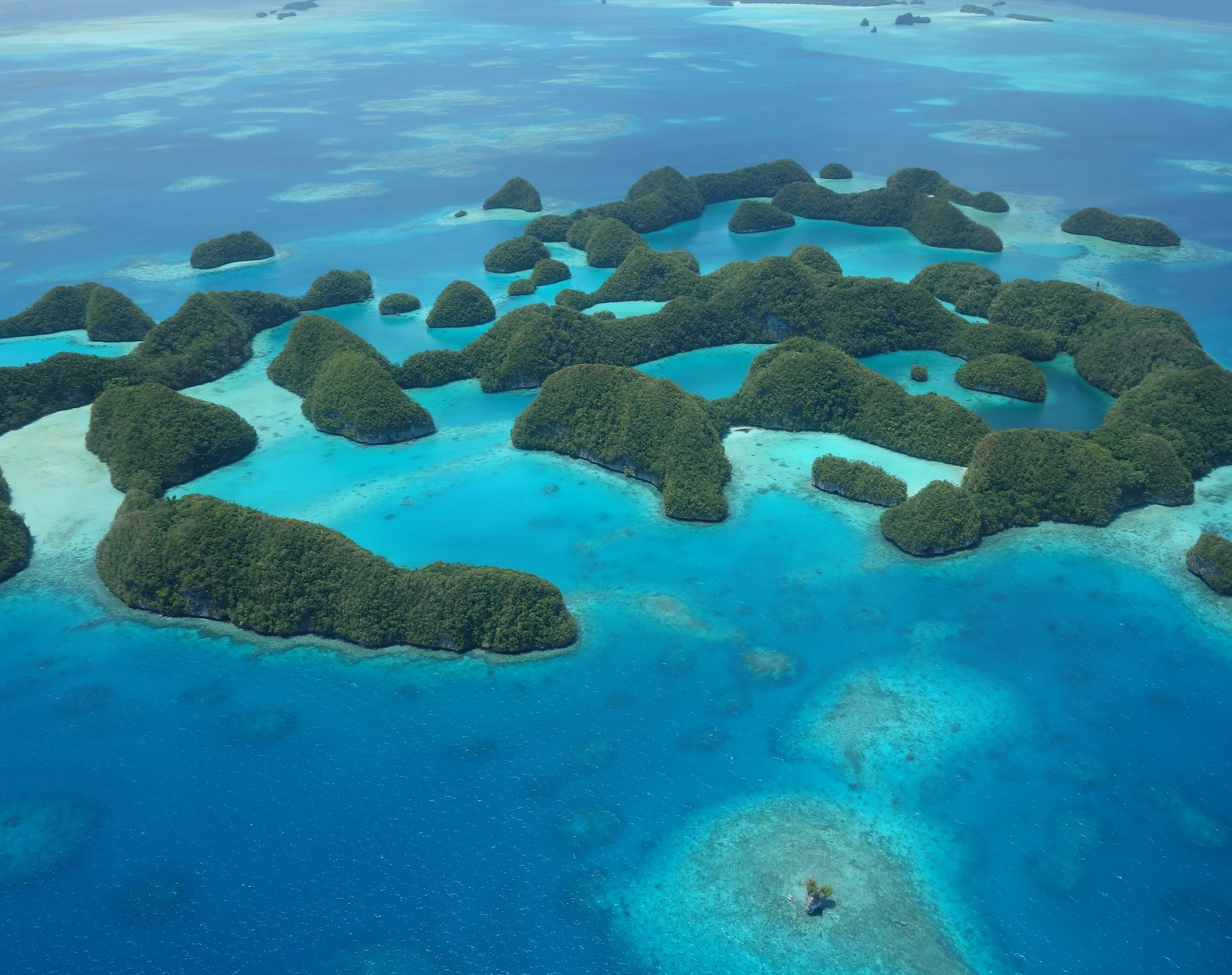
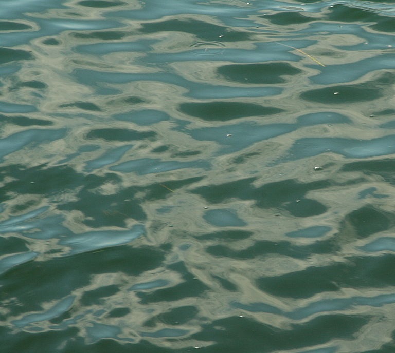
Whether the goal is realism or fantasy, the purpose of noise is generally the same: to mimic patterns in nature. One of nature’s fundamental properties is isotropy, or the even distribution of patterns regardless of angle. Nature doesn’t have a grid, and it doesn’t pick any directions as favorites. It’s worth being able to explore one’s terrain, for example, to find cliffs, mountains, valleys, and coastlines that follow many directions rather than primarily those on a compass rose. Procedural primitives that capture this effectively fulfill more of our visual expectations, and immerse us better in the end result. Directional uniformity is as central to the role noise plays in procedural generation as the curvature itself is.
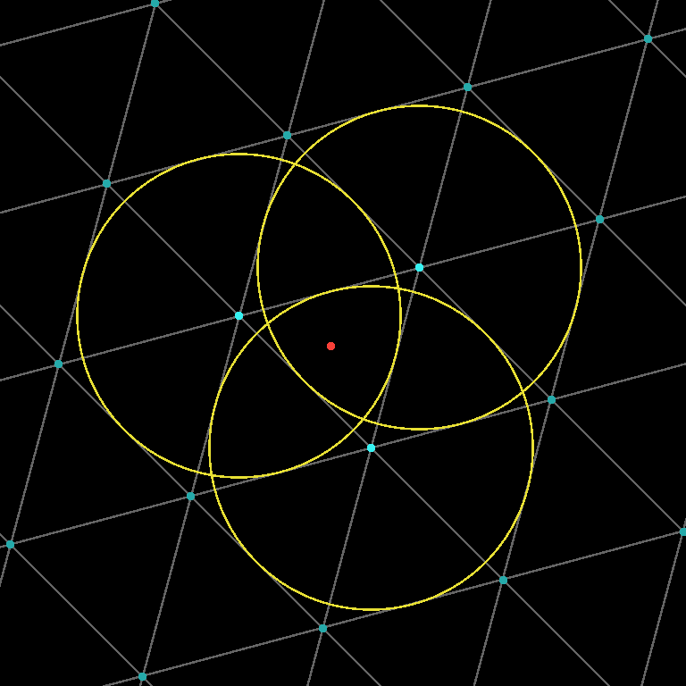
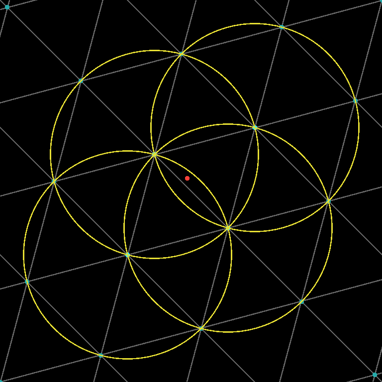
What Causes It?
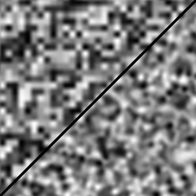
The Perlin noise algorithm is based on a square, cubic, or in general hypercubic grid. On each vertex of this structure, it chooses slope directions (gradient vectors), computes their extrapolations, then mixes them together with their neighbors. Its bias is a straightaway consequence of this arrangement, and how the gradients interact on it. New gradients only come in at grid vertices, and their bumps only join together across vertices of the same cell. Features with grid-favored angles merge with no effort, while those with the rest aren’t often so successful. The resulting patterns adhere to the grid, thereby following the coordinate directions which form its basis.
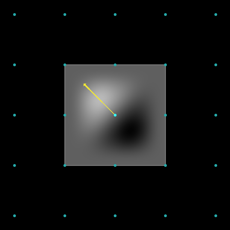
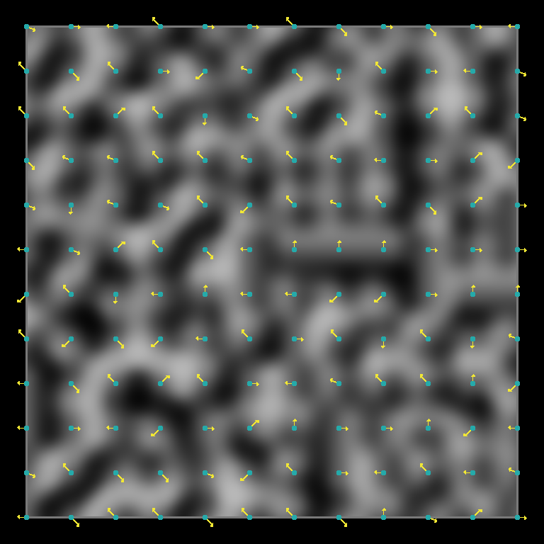
Uses 2D slice of 2002 “Improved Noise” gradients.
Click here to see one using a more-uniform 2D set.
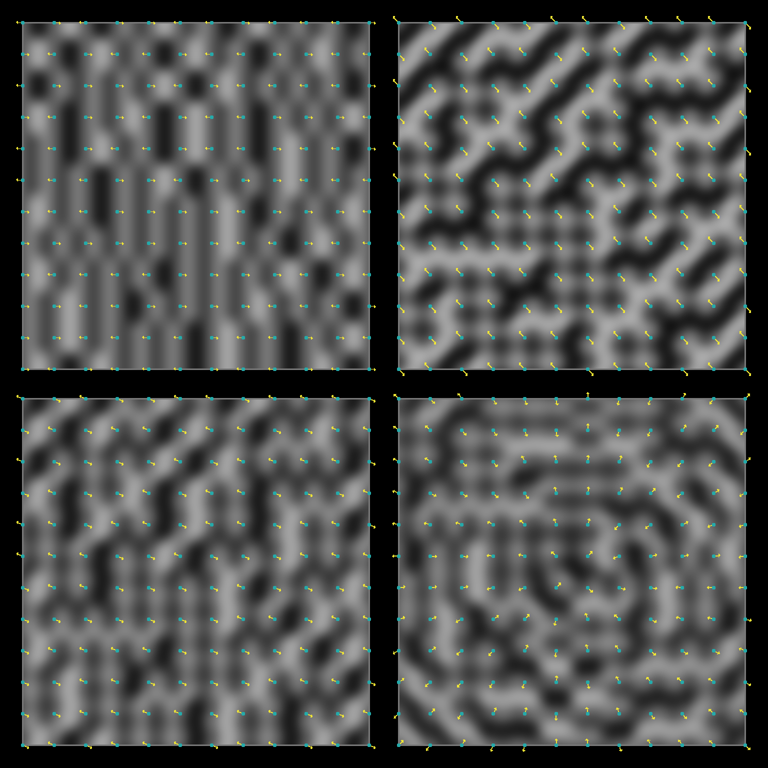
Horizontal (◰), 45-degree (◳), 22.5-degree (◱), circular (◲).
Not Just Perlin
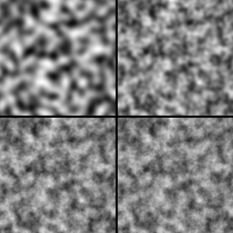
Perlin has found itself at the forefront of the noise conversation for a while now, so it makes sense to address the problems it has in specific context of it. That doesn’t mean that there aren’t others that share its issues, though. Value and Value-Cubic noises, found in many libraries themselves, falter through their use of the same grid structure. While they exhibit different characteristics which lend them to different use cases, their related shortcomings warrant similar critical light.


Value noise displays the most prominent artifacts, resembling a blurred pixel grid with clearly recognizable cells. It’s certain, at least, what Perlin has in looks over Value; nonetheless they both look square. Value-Cubic produces more-varied features, but it still struggles to decouple them from the grid layout. Later in the article, I’ll circle back to how we can improve the looks of all of these noises. First, though, I’ll cover an alternative that you might already know.
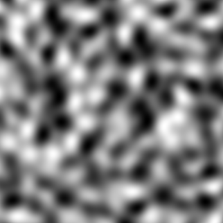
Simplex(-type) Noise
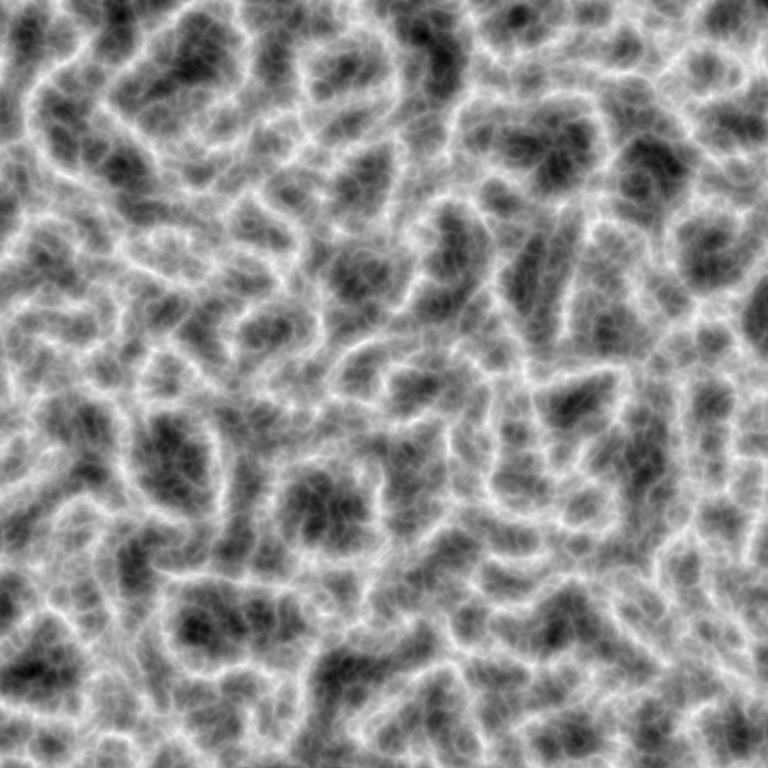
If you’re familiar with any of the noises above, you may have also heard of Simplex noise. Simplex noise is a second algorithm by Perlin noise’s eponymous author, that was put forth as a successor to his original algorithm. One of its primary selling points is its reduction of visible directional bias through the use of a new grid structure. In this section, I’ll examine this noise, tie in some of my own contributions to the space, and illustrate why noises like this have certain elementary advantages over Perlin and Value that mark them as better standards.
Expired Patent, Related Noises
Those of you familiar with Simplex may also know of its US patent (US6867776B2), which covered certain implementations and use cases of the noise in 3D+. While thankfully somewhat refined in scope, it surely played a role in curbing the noise’s popularity. In efforts to alleviate some of these concerns, I introduced OpenSimplex (2014), then OpenSimplex2 (2019) and OpenSimplex2S (2017/2019). These noises gained some traction in applications that would otherwise use Simplex. All four of these Simplex-type noises share key details, both inside and out, that relate them to one another.
Inner-Workings
Simplex, the namesake of the noise, refers to the shape in a given number of dimensions with the lowest possible number of vertices. In 2D it’s a triangle, in 3D it’s a tetrahedron (or triangular pyramid), and in general it has just one more vertex than the number of dimensions. These noises are characterized by their use of grid schemes based on these rather than squares or cubes. Grids like this provide more basis directions, decouple themselves from the coordinate axes, reduce the maximum possible misalignment of any given observation angle, and generally pack the vertices together more tightly. This adheres them more tightly to the principles founding noise generation, and attunes them better to what we use them for.
Simplex-type noises attach gradients to each vertex in much the same manner as Perlin, but combine them differently. Instead of interpolation, they use spherically-bound functions for contribution falloff, which are more portable to arbitrary point layouts. The gradients ramps are added to the final noise value, each multiplied by a weight that depends only on the distance to the vertex it comes from. At the sphere boundary, that weight becomes zero, and the gradient no longer contributes. This scheme is shared across these algorithms, whose main differences become the grid constructions they use and how they determine which points are in range.
Do I need to understand all that?
No, not generally. A firm grasp of the inner functionality can be instrumental towards modifying an algorithm, debugging one, or implementing one yourself. It can also be rewarding as a programming and mathematical exercise, and can enable you to create specialized variants where you need. However, it isn’t a requirement for ordinary use of the noise. There are numerous freely-available open-source libraries that are well-documented, straightforward to import, and support good quality Simplex-type noise. Libraries get the heavy lifting out of the way, so you only need to worry about what you actually do with the noise.
Algorithms & Implementations
All of these noises exhibit crucial similarities, but not all variants are created equal. Gradient sets and contribution radii both serve to set one adaptation apart from another.
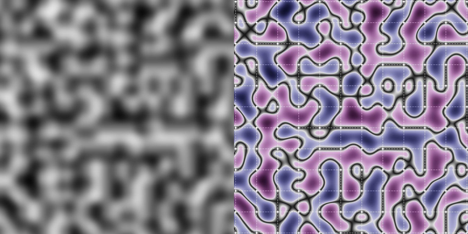
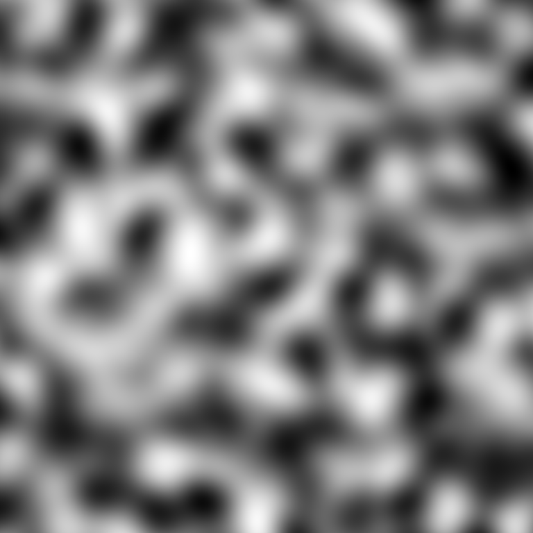
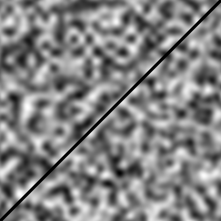
A gradient set is the space of possible slope directions that can be assigned to each vertex on the grid. Good sets promote visual isotropy and avoid isolated tall bumps that throw off the noise’s value range. Some older Simplex implementations used less-tuned gradient sets which allow some squareness to sneak back in, so it’s worth looking out for their artifacts.
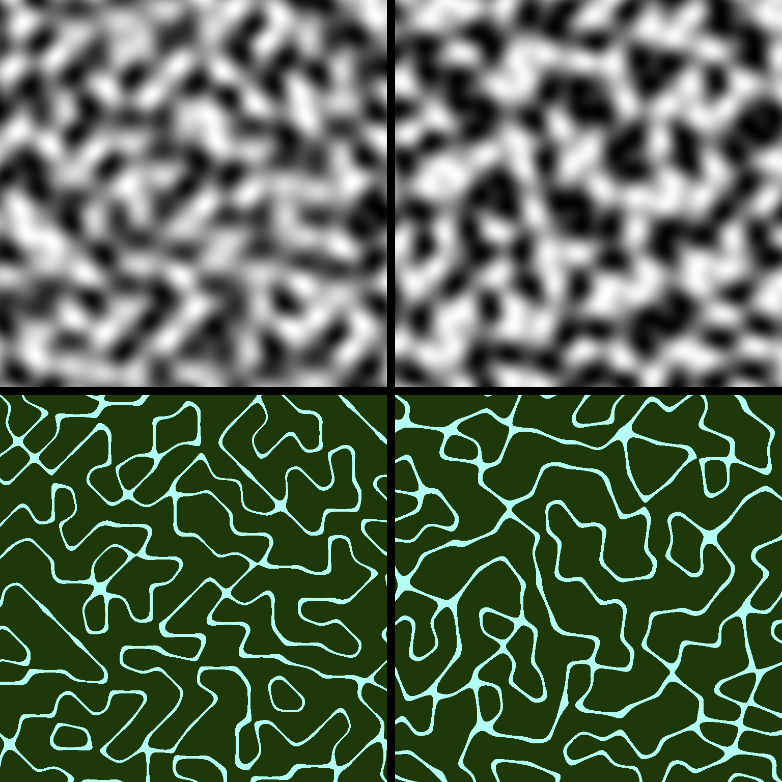
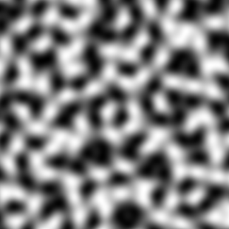
Noise with original gradients (◰); with 24-set (◳).
Contours around zero with original (◱); with 24-set (◲).
Same noise with re-oriented gradients (right).
(We’ll get to this shortly!)
Contribution radius, the primary difference that sets OpenSimplex2S and 2014 OpenSimplex apart from Simplex and OpenSimplex2, affects the contour behavior and overall shape of the noise. Ridged fractal noise, in particular, benefits from softer curvature yielded by a larger radius. These two algorithms aren’t as fast, however, as they require adding together more vertex contributions.
Smaller differences in contribution radius can also be found between some 3D+ implementations of Simplex and OpenSimplex2. The original Simplex paper called for R² = 0.6 and dimension-specific tuning, while the technically-correct, discontinuity-avoiding constant is always R² = 0.5. Nonetheless, the small-order jumps in value are undetectable in most ordinary use cases.
R² = 0.6 vs R² = 0.5 in 3D OpenSimplex2 noise.Domain Rotation
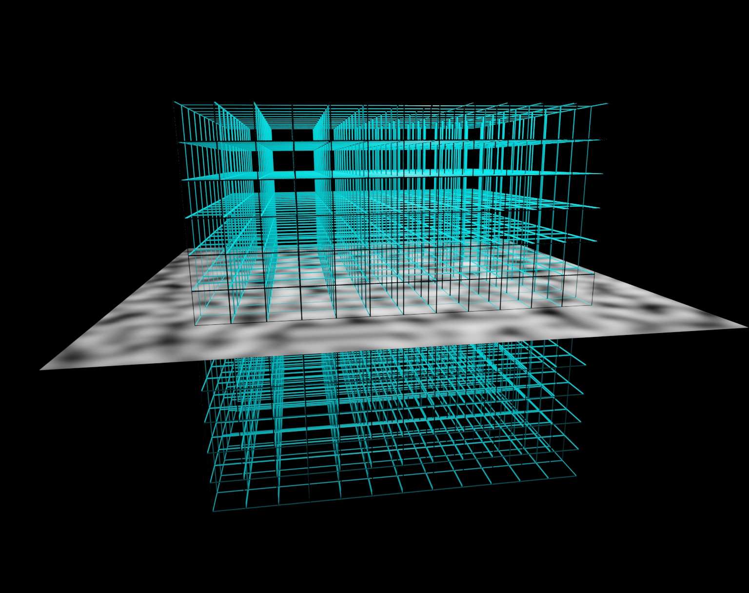
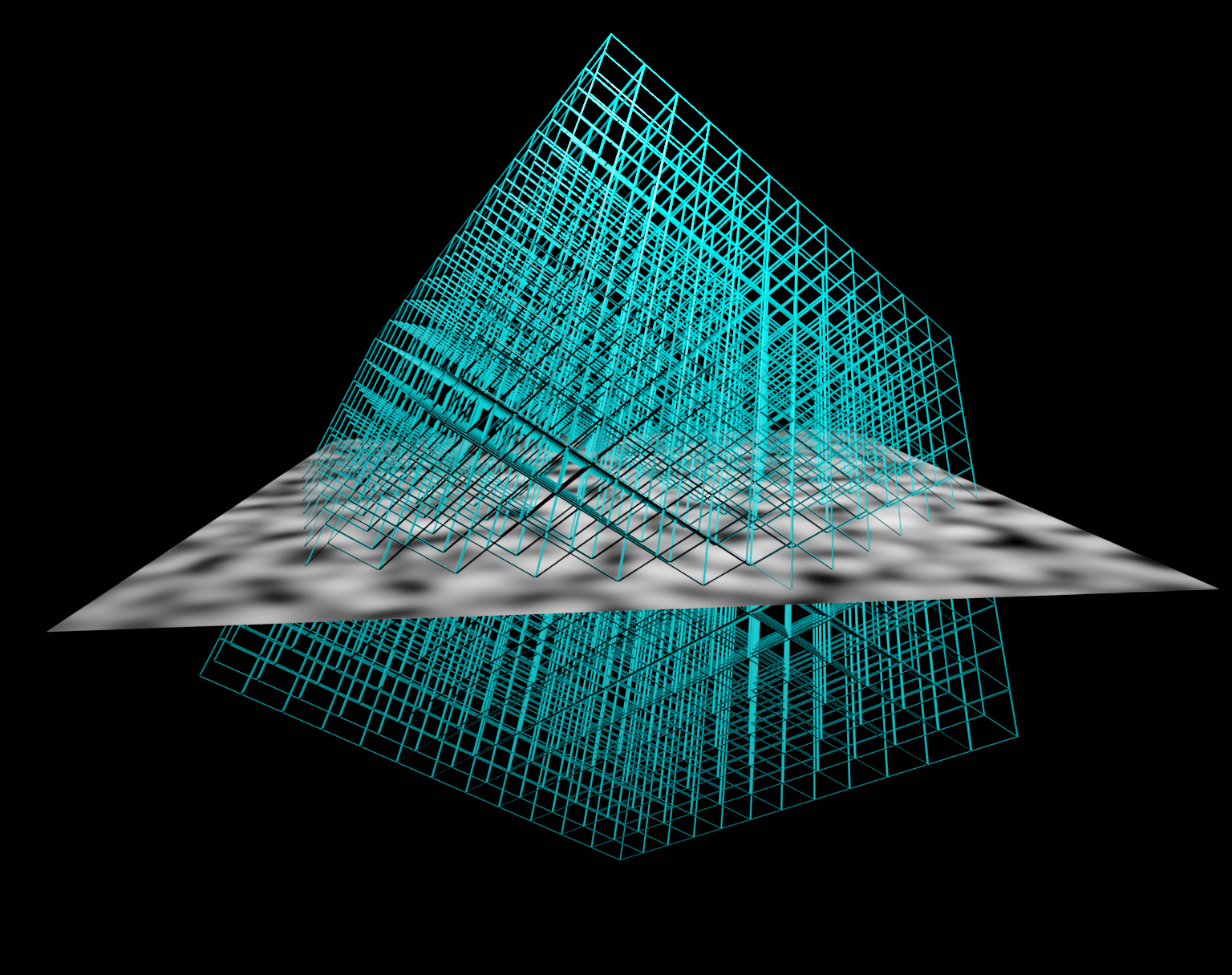
In the section above, I discussed the ways Simplex and its relatives improve visual isotropy in comparison to common cube-grid-based noise algorithms. Here, we’ll find out that switching the algorithm isn’t necessarily the only route to a dramatic improvement. A surprisingly effective technique, seemingly first showcased at the bottom of an article written in 2014 by Catlike Coding, is to rotate the sampling space of the noise. Not to be confused with Domain Warping, this Domain Rotation involves transforming a noise’s input coordinate via a linear rotation transform. The proper rotation used in the right circumstances can cause the griddiest parts of a noise to disappear from the cross-sections observed. The article didn’t dive far into detail or reasoning, so I’ll cover it more comprehensively here.
Dimensions and Ideal Rotations
The first thing to know when rotating noise to improve its look is that you need at least 3D noise. Indeed, when filling a 2D plane with 2D noise, there is nowhere for the artifacts to go. The noise will just rotate within the plane, leaving its patterns as exposed they were as before. But by using 3D noise, it becomes possible to define rotations that altogether move its internal square planes out of alignment with the observer’s view.
The definition of such ideal rotations goes as follows: Choose one coordinate that will point up the main diagonal of the noise grid. Typically in 3D, this will be Y or Z, but it could be any we choose. By deriving a rotation that satisfies this mapping, the rendering plane takes a much nicer looking slice through the noise.
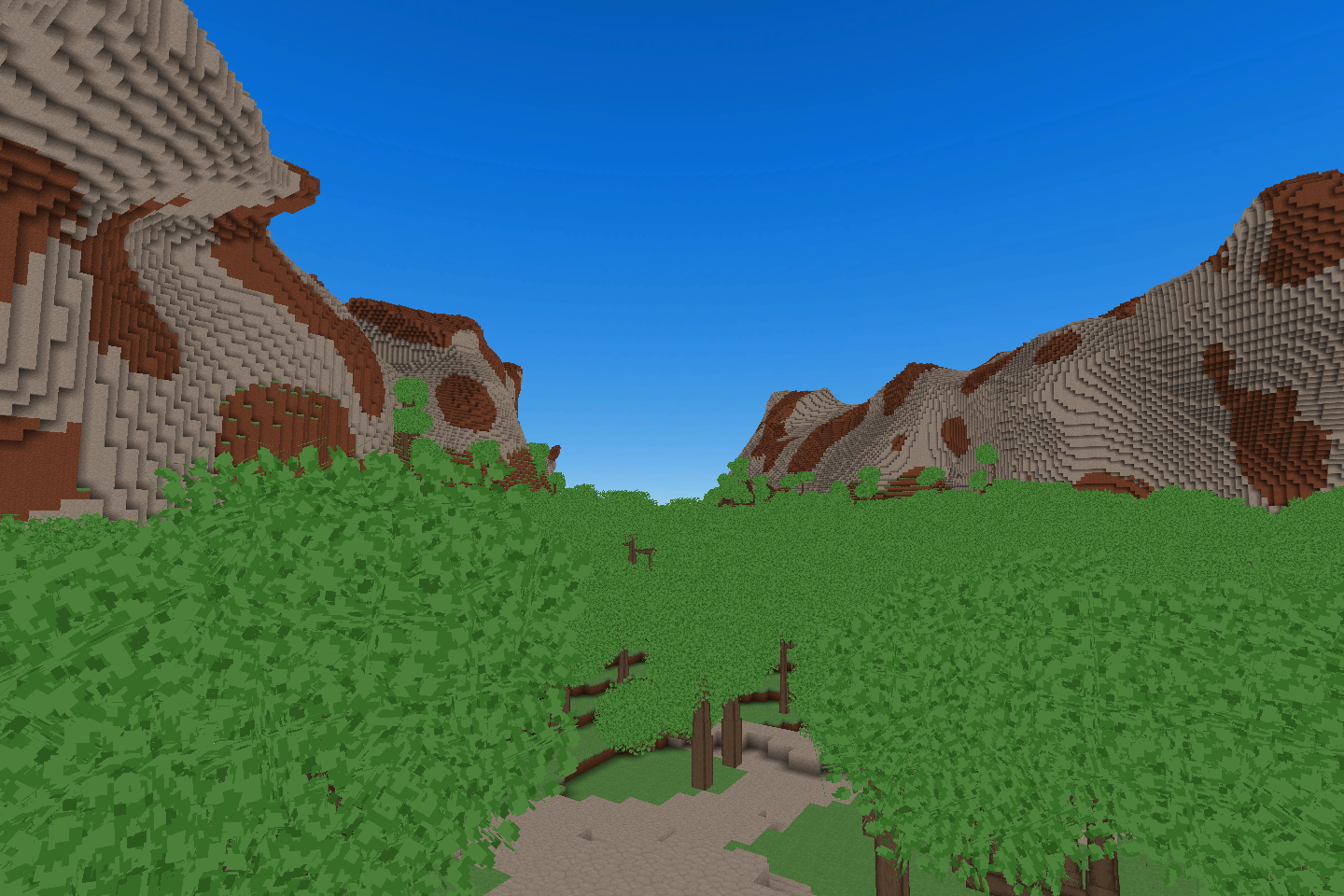
Now it would seem, in general, that we always need one dimension higher (N+1) to produce good N-dimensional noise. This is true for 2D, and might be proper in many 3D situations such as texturing spherical planets. In such examples, Simplex-type may be the better fit anyway. However, in certain cases, we can attain the full benefit using only the same dimensionality of noise. 2D-focused use-cases of 3D noise, including overhanging voxel terrain and time-varied animations, are prime examples of this. In these scenarios, the third dimension plays more of a supportive role, and can be assigned to the main diagonal direction without issue. This is where Domain Rotation truly shines, because we can realize its value with virtually no performance penalty.
(note: lighting improvements on hold)
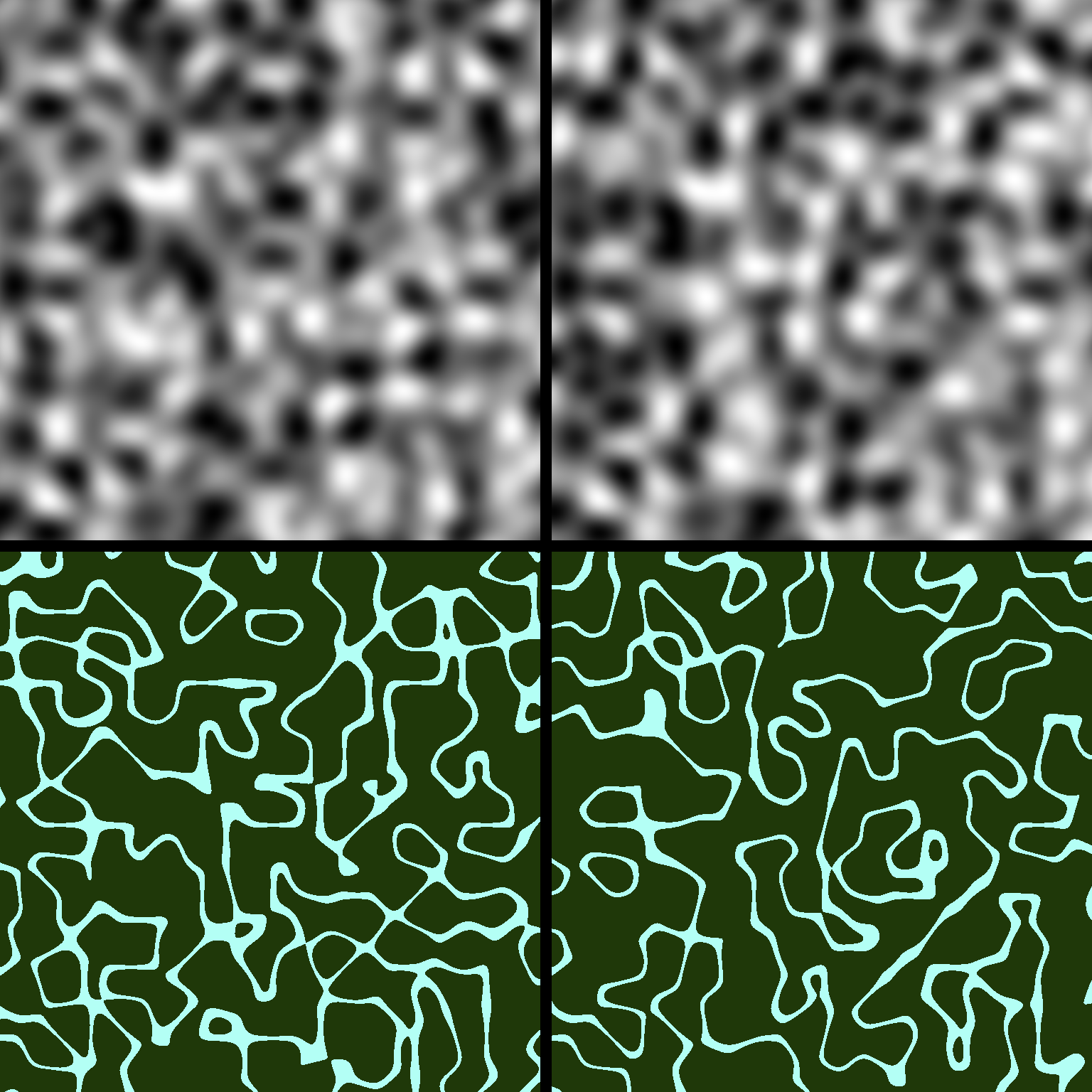
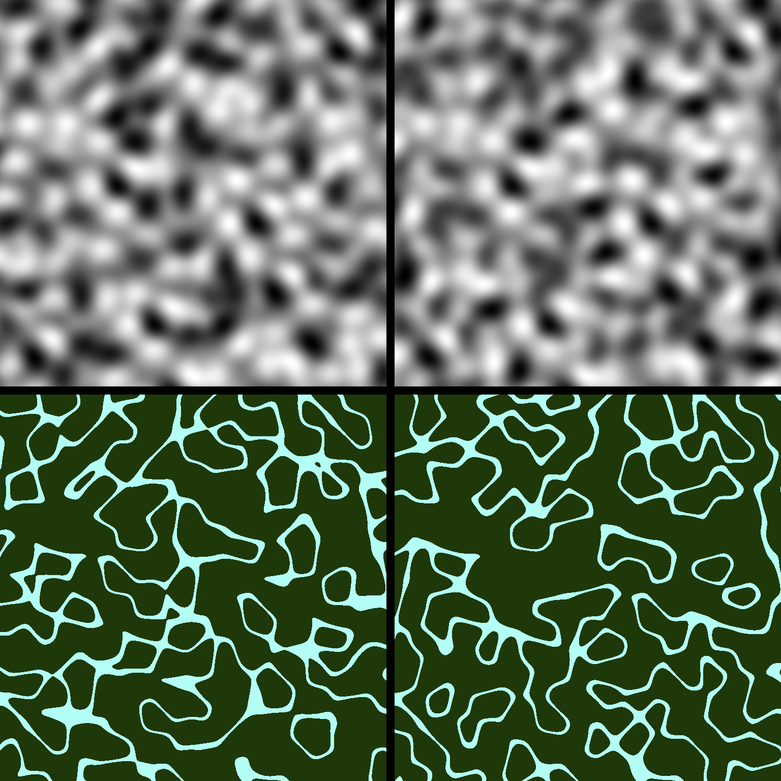
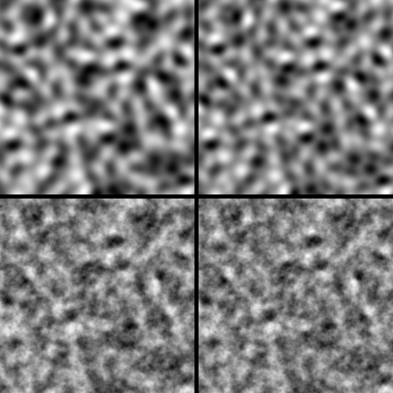
Results
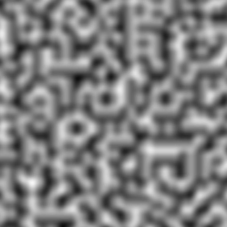
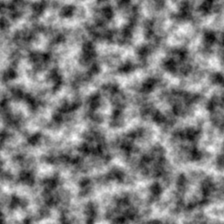
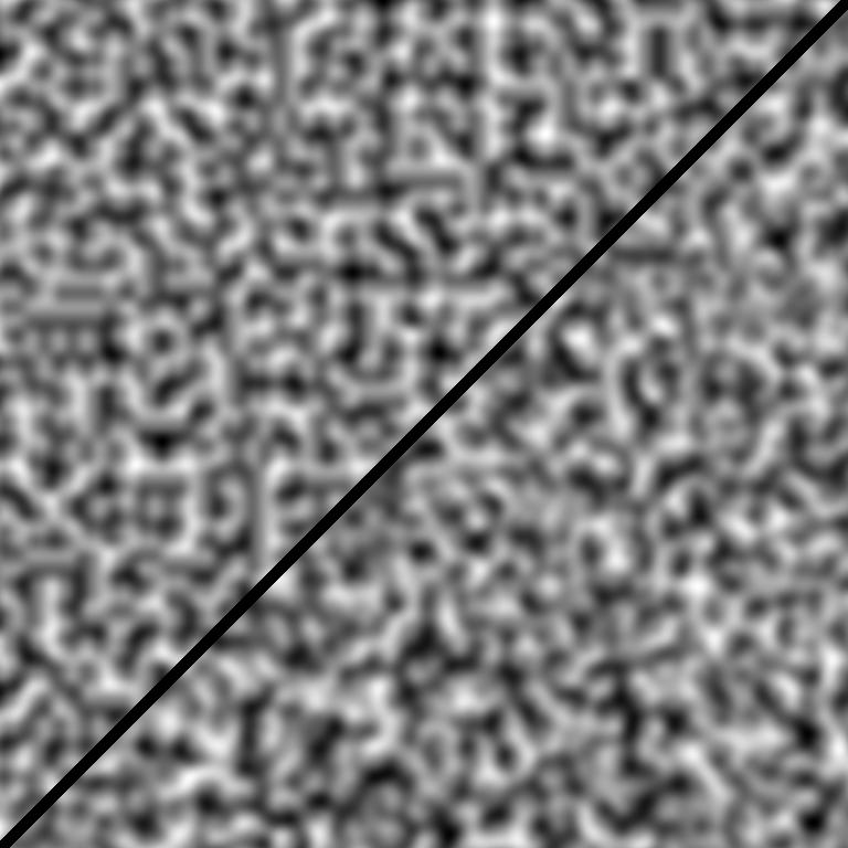
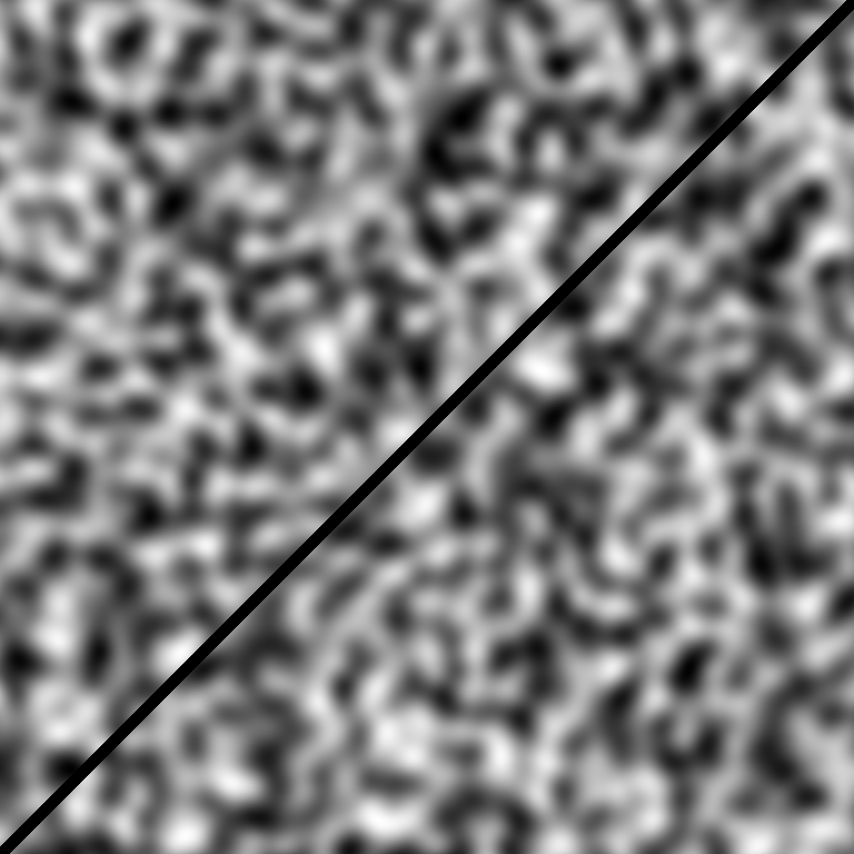
Illustrating this domain rotation on the three cube-grid algorithms, its effects become clear. Square bias disappears from all three noises, preserving varying other aspects of their character. Perlin sees only modest change in overall appearance, in exchange for a substantial reduction in discernible alignment.
Value noise experiences an extravagant transformation, though it still isn’t the cleanest contender. Value-Cubic retains much of its composition, but sheds its grid-founded perforations.
It even works on Simplex and co. to clear up some slight probabilistic asymmetry, though the difference is a little hard to tell here. In truth, I rendered most of the 3D Simplex-type noise figures in this article using this rotation.

Formula
Here, I will go into the derivation of the formula for the 3D rotation. You can skip over this if the technical details aren’t particularly important to you. I’ll link a library that offers an implementation of this at the end of the article. I will likely also write an article in the future that covers more of the odds and ends of this topic, both practically and mathematically.
As hinted at the beginning of this section, rotations are linear transforms. This means they can be expressed as matrices, or equivalently by assigning new vectors to each old coordinate direction. For example, Y without rotation moves along <0, 1, 0> in the noise. We want to pick new vectors for each coordinate that move them in the directions we would like.
Noise domain rotation will typically single out one coordinate to be treated differently than the rest, e.g. as the vertical, time, or unused direction. The rest will then, ideally, behave symmetrically to each other w.r.t. the noise grid, so as to simplify convention. The first step is to send this “special” coordinate (e.g. Z <0, 0, 1>) up the main diagonal of the noise grid. The vector <1, 1, 1> moves in the direction we want, but it’s not unit-length. Using a different magnitude changes the frequency of the noise, so to counter that we will divide by its magnitude to get the unit vector we can assign to Z. <1, 1, 1>/length(<1, 1, 1>) = <1, 1, 1>/sqrt(3) = <g, g, g> where g ≈ 0.577350269189626. Note that we don’t need to compute any square roots at runtime, just during development to determine what the vectors should be.
Then to assign the right vectors to X and Z, we want to pick two that are (1) 90 degrees to the vector we just created, (2) 90 degrees to each other, (3) also unit length, and ideally (4) symmetric to each other on the noise grid. It turns out that, because the cross-sectional point layouts of an N-dimensional hypercubic grid where x+y+z is an integer are equivalent to the grid structure used in 2014 OpenSimplex, we can just borrow its skew constant s = (1/sqrt(N+1)-1)/N (≈ -0.21132486540518713 for N=2) – which itself is a borrowing of the unskew constant from original Simplex. Then we can choose h in X: <1+s, s, h> and Y: <s, 1+s, h> to make them 90 degrees to <g, g, g> (or equivalently to <1, 1, 1>). To our luck, it will turn out that g = -h and also that the resulting vectors themselves are unit length.
Writing this out: x*<1+s, s, -g> + y*<s, 1+s, -g> + z*<g, g, g>, we see some opportunity for simplification. xr = (1+s)*x + s*y + g*z, yr = s*x + (1+s)*y + g*z, zr = -g*x + -g*y + g*z. xr = x + (x+y)*s + g*z, yr = y + (x+y)*s + g*z, zr = g*z - (x+y)*g. Then we can write A = g*z, B = x+y, C = B*s + A so that xr = x + C, yr = y + C, zr = A - B*g, and that’s what we can use to transform our noise coordinates. Here it is in code:
public static void noise3_ImproveXZ(double x, double y, double z) {
	double xz = x + z;
	double s2 = xz * -0.211324865405187;
	double yy = y * 0.577350269189626;
	double xr = x + (s2 + yy);
	double zr = z + (s2 + yy);
	double yr = xz * -0.577350269189626 + yy;

	// Generate noise on coordinate xr, yr, zr
}
Here is the same transform implemented for 4D, choosing the W coordinate:
public static void noise4_ImproveXYZ(double x, double y, double z, double w) {
	double xyz = x + y + z;
	double s3 = xyz * (-1.0 / 6.0);
	double ww = w * 0.5;
	double xr = x + s3 + ww, yr = y + s3 + ww, zr = z + s3 + ww;
	double wr = xyz * -0.5 + ww;

	// Generate noise on coordinate xr, yr, zr, wr
}
You can also chain rotations for successively lower dimensions. Here is an example of that, combined and simplified:
public double noise4_ImproveXYZ_ImproveXZ(double x, double y, double z, double w) {
	double xz = x + z;
	double s2 = xz * -0.21132486540518699998;
	double yy = y * 0.28867513459481294226;
	double ww = w * 0.5;
	double xr = x + (yy + ww + s2), zr = z + (yy + ww + s2);
	double yr = xz * -0.57735026918962599998 + (yy + ww);
	double wr = y * -0.866025403784439 + ww;

	// Generate noise on coordinate xr, yr, zr, wr
}
Conclusion
Perlin noise has problems with squareness which run at odds with its purpose. Good implementations of Simplex and its relatives represent better standards, and Domain Rotation addresses its issues in place.
It’s important to consider modern knowledge on a subject when incorporating a tool into our workflows. Old unmitigated noise finds its way into more new things than it belongs, in light of our options now.
This article presents counterpoints to a particular regression that many sources reiterate. The follow-up article will carry this further, suggesting ways we can work to improve the state of information on this topic through careful consideration of what we teach.
Extras
Don’t these solutions just replace square bias with hex bias?
Yes and no. The resulting grids (or planar cross-sections) do follow some hexagonal trends, but the added basis directions combined with lack of cardinal axis alignment function to make them less obvious. Simplex-type noise and domain rotation aren’t perfect, but they’re among our best options today for visual isotropy within the performance bracket we expect.
What if I use the biased noise for stylistic reasons?
The first question I would ask would be if the bias itself is part of the style you’re going for, or if there are other parts of its character that serve as truer reasons. If the latter is the case, a good general principle would be to isolate the favorable parts in the solution. Domain Rotation, as covered here, is a great tool for this in noise. If you’re using the bias itself for style, then the remaining question would become how your creation sets itself apart from the sea of those where it’s evidently a side effect.
What if my world is made of blocks or tiles?
A tempting thought might be: If a game is based on a grid of blocks or tiles, would it not make sense for the terrain to follow that grid? It sounds like a logical parallel, but it can also serve as an intuition trap. My primary reason for not subscribing to this notion relates to differentiation between scales.
At what scales should should the block/tile layout influence the world’s form, and in what ways? Should the shape of a vast continent be a consequential product of its small representational elements? What grid-biased behavior really actually belongs above the scale of the actual block/tile grid? Perhaps world generation using these building primitives is less about extrapolating their underlying geometric structure into larger trends, and more about making great artistic/visual use of the pieces – especially where nature-inspired curvature is already in play. Like an image made of pixels isn’t forced to follow its own grid, worlds made of blocks or tiles need not remind us of any coordinate-space math under the hood. The aesthetic charm of the tiles/blocks is self-evident, leaving worlds built upon them free to follow whatever rulesets put them to the best overall use.
What if the player never sees an aerial view?
The vantage points from which your players observe the world, and what they reveal about it, are worthy and valid considerations when setting priorities during development. It’s possible a player will notice different issues at ground-level versus flying high above. However, visual anisotropy can manifest in many perspectives, and it may not be just the player camera’s point-of-view to account for. In-game maps, promotional material, and possible community-made mods/tools all have potential to showcase the world in different ways, so it can be worth considering how it looks from many possible angles. It’s a straightforward win on attention to detail, where the solutions are already readily available.
What if my framework already offers just a Perlin/Value function?
Unity and P5.js, for example, offer noise options that are conveniently-accessible, but poor in quality and directional variety. For Unity, it’s Mathf.PerlinNoise, and for P5.js it’s the fractal-Value-mislabeled-Perlin noise module. My first step when using platforms like this, whether for my own development or as teaching utilities, is always to import an external noise library. Hopefully, in the future, the teams and leaders behind tools like this will come to understand the ways this skews the product space, and push updates to improve the situations. For now, though, we at least usually have the ability to pull in alternatives ourselves.
How does the Diamond-Square algorithm play into this?
Diamond-Square is a terrain/texture method early in origin, which involves recursive midpoint value displacement on a pixel grid. The finer-grained control it offers has been praised as a strong point, but it loses out in significant ways on quality and directional variety. The effective calculations it performs aren’t unlike fBm Value noise under plain linear interpolation, and its visual results turn out likewise with grid-aligned creases.
What about one-dimensional noise?
Visual isotropy doesn’t become a proper concern until you hit at least 2D, so from that standpoint all choices are essentially equal. But perhaps from a different perspective, it might be worth finding a noise that doesn’t cross zero on regular intervals the way the 1D generalizations of Simplex or Perlin do. The simplest way to solve this is to sample a line or path through 2D noise of any type, avoiding any points or vertices that are zero by definition.
Libraries
- FastNoiseLite - Straightforward library for common use cases or for getting started, that supports OpenSimplex2(S) noise as well as 3D domain rotation through a configuration option.
- FastNoise2 - Hyper-optimized SIMD-enabled library with support for Simplex-type noise and an angle-based rotation node*.
- OpenSimplex2 - My own repository that serves as a home base for OpenSimplex2(S) noise.
- WebGL noise - GLSL implementations of noise functions including Simplex.
* 3D-only. Use Euler angles -0.2617994, 0.6154797, -0.7853982 for XY-horizontal, or -0.6319143, 0.2129302, 0.6319143 for XZ-horizontal.
Resources
- BIT-101: Perlin vs Simplex
- Red Blob Games: Making Maps with Noise Functions - Comprehensive, recurrently-updated noise fundamentals article presenting primarily-modern* information.
- Stefan Gustavson: Simplex Noise Demystified
- Ken Perlin: Noise Hardware - Original Simplex noise paper.
* The accordingly-named section in Making Maps with Noise Functions contains links to several implementations of noise. The mentioned Unity Mathf.PerlinNoise function can work for simple experimentation, but is difficult recommend beyond that. The linked libnoise library offers a rotation node, but is missing support for Simplex-type noise, teaches several terms incorrectly in its documentation, and has not been updated since 2007. The article itself is a great introduction to the application of noise to terrain generation.
Proofreading Credit (original article)
- YUNGNICKYOUNG
- Amit Patel (Red Blob Games)