Mar 22, 2021
One of the trickiest steps that can be involved in implementing noise algorithms is to make their output fit tightly into certain bounds. Generally, this is accomplished by determining the min and max of the unmodified noise as accurately as possible, then rescaling the output to [-1, 1]. There is not always a nice formula to compute these values, and brute-force approaches can be unreliable. In this article, I will describe the tools I created to find these values in common gradient-based noises, and the techniques they employ.
Purpose
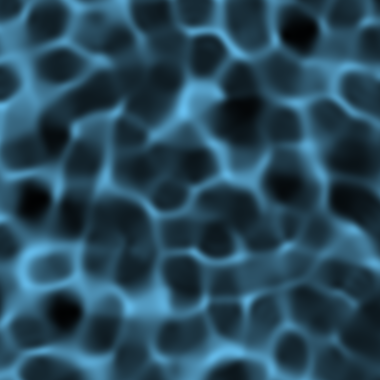
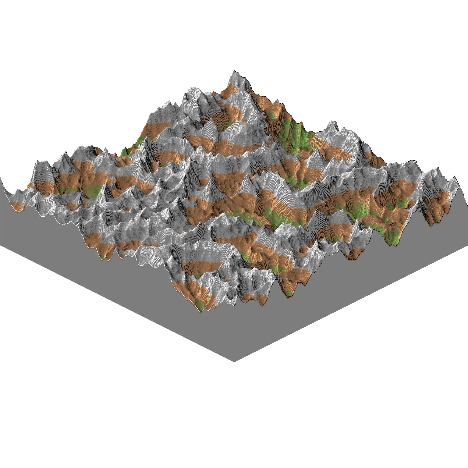
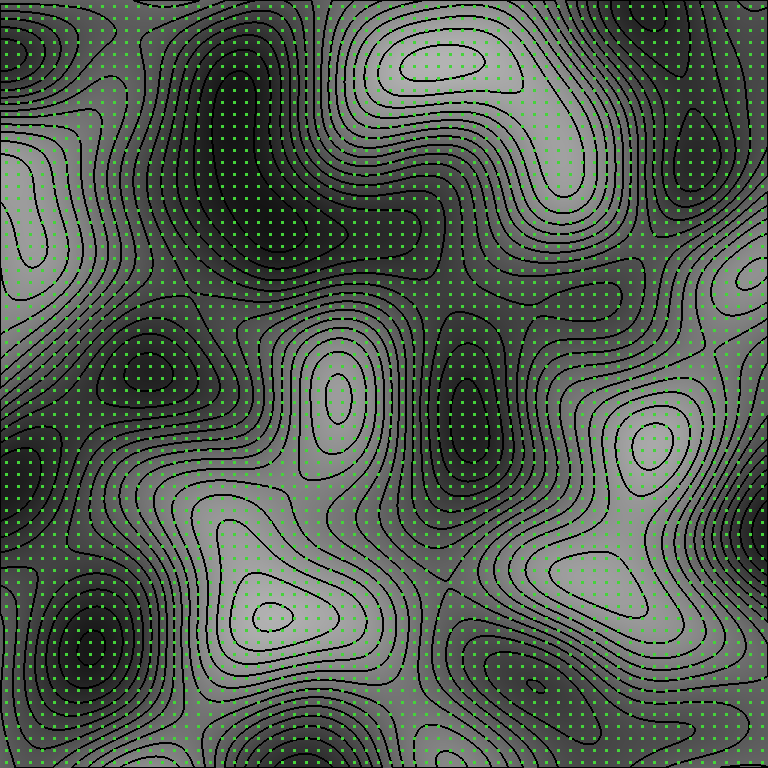
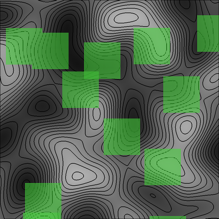
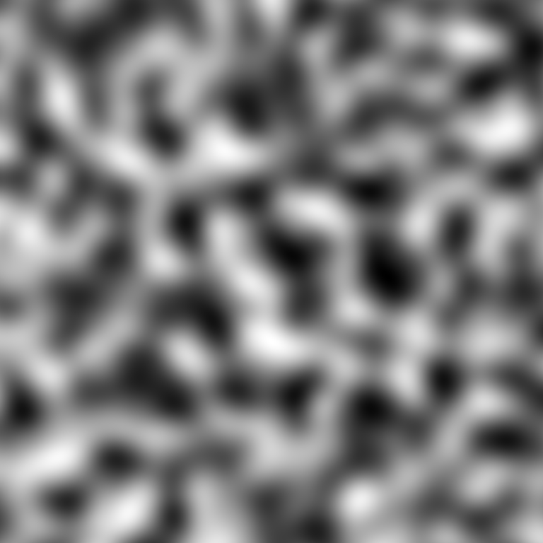
Noise is used to generate many effects in textures and terrain. In textures, knowing the noise bounds can help the developer or artist accurately control the color ranges produced by its variation. In terrain, consistent bounds can help establish accurate height ranges. There are also many ways in which noise layers are combined, and many formulas noise can be passed into, which depend on its values not exceeding certain numerical boundaries. It is common for users to expect noise to fit a range of -1 to 1, though this can be difficult to implement accurately.
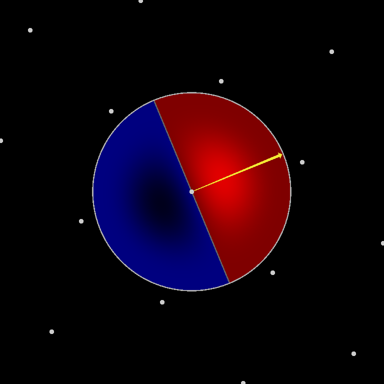
Symmetry About Zero
Gradient noise algorithms, in their most common forms, naturally produce value distributions centered around zero. This is due to three main reasons. First, each gradient ramp begins at zero on its respective grid vertex. Second, due to the symmetric shape of its contribution range, it contributes exactly as much on its positive side as on its negative side. Finally, for any positive value that occurs, it is always possible for its negative to occur somewhere, and vice-versa. This fact comes most intuitively when every possible gradient has a sign-flipped counterpart within the set of available vectors (e.g. <1, -1, 0> and <-1, 1, 0>), but it is also guaranteed by grid symmetry. It follows that min=-max, and it suffices to find just one of the two.
Brute Force
A simple approach might be to evaluate the noise billions of times at random coordinates, and keep track of the maximum absolute value it produces. This can produce close results, but it presents three main problems. First, the true maximum can be incredibly rare in some noise, even if local maxima come close. Second, even if you regularly land near a maximum, it is unlikely that your evaluation point will coincide accurately with it. Finally, an inaccurate result is always smaller, which makes it a poor choice for a bound. padding the value to contain the entire noise range is then left as guesswork to the developer.
The random coordinates can be replaced by a grid of regularly-spaced coordinates, however this suffers similar problems. If the grid is distributed over a large area, then it is likely that no evaluation will be close to the maximum. If the grid is compressed into a small area, any local maximum will be returned more accurately, but there is less chance of the global maximum occurring in that area. Even with a hybrid approach, the grid resolution would need to be very high to generate a result that would not require any padding.
The rarity problem can be further understood as follows. Each noise grid cell sees contributions from some surrounding vertices. A cell might only contain the global maximum (or minimum) if its gradients are aligned just right. If a noise uses 24 gradient options and 3 contributions per cell, there would only be 24^3=13,824 possibilities (not adjusting for symmetry). In this case, you are at least likely to visit the optimal cell configuration many times over. But if a noise uses 48 gradients and 8 vertices, it might have on the order of 48^8=28,179,280,429,056. Even with 8 ways to mirror the gradients, plus a sign flip, that’s still a 1 in 1,761,205,026,816 chance that any given cell will contain the maximum.
Exact Formulas
An idealized solution might consist of expressing the exact result in terms of functions that are available in common mathematics libraries. On paper, this feels like a noble goal. However, a number details get in the way.
High-Degree Polynomials
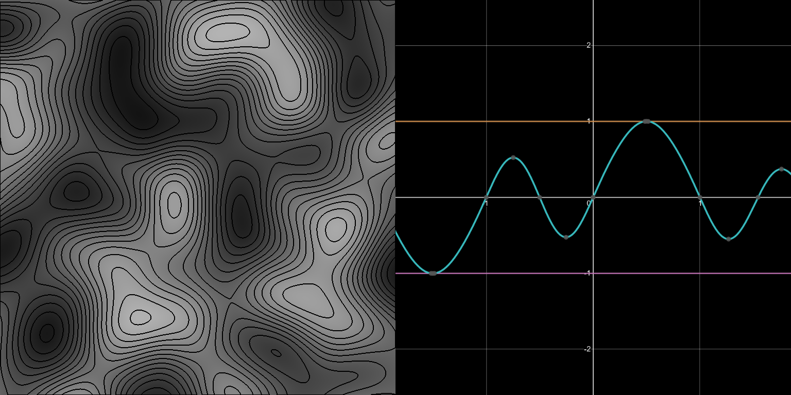
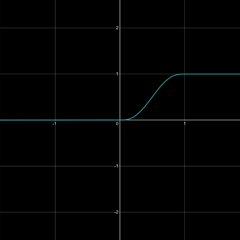
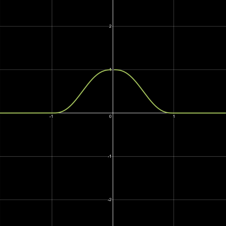
Common gradient noises all involve, in some form, piecewise polynomial functions that define contribution falloff weights for each grid vertex in range. Each weight is multiplied by a gradient ramp emanating from the vertex, and the results are combined to form a final noise value. This might sound complex, but it’s really just the combination of a few simple math functions. The graphs below illustrate what happens. Note that the max(...) component, which prevents the function from dropping below zero, is what characterizes the falloff function as piecewise.
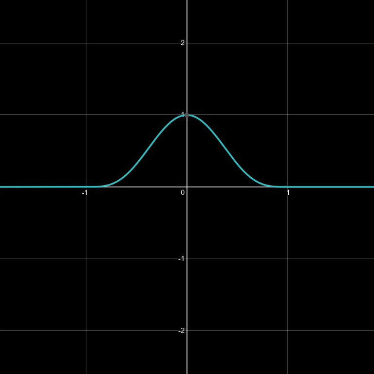
w(x)=max(0, 1-x^2)^4 (all graphs plotted using Desmos)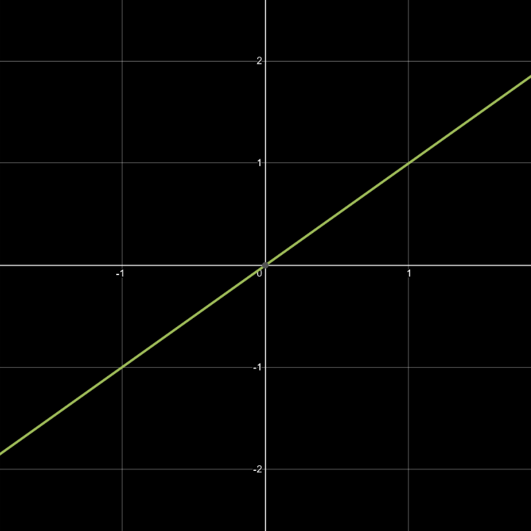
g(x)=x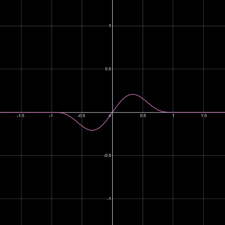
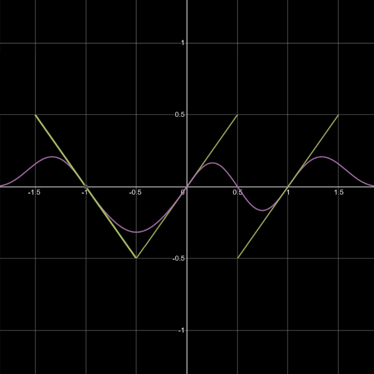
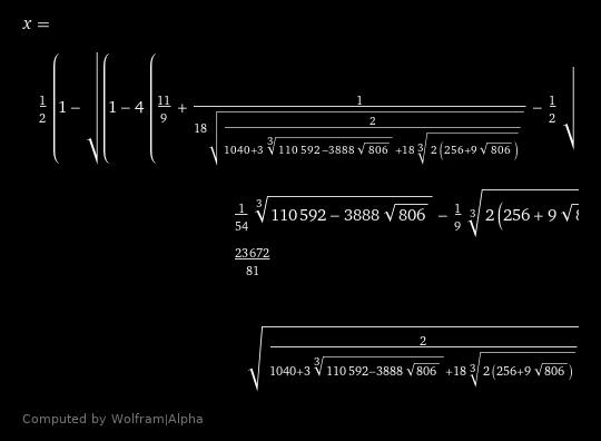
Even if we ignore the piecewise aspect, solving for the local minima or maxima of these high-degree polynomials is not always easy. According to Galois theory, it may not even be possible without introducing additional functions not available in common mathematics libraries. Even though simplified cases like these may be solvable, the expression can be quite gnarly. This also doesn’t cover what happens when additional dimensions are introduced.
Gradient Sets
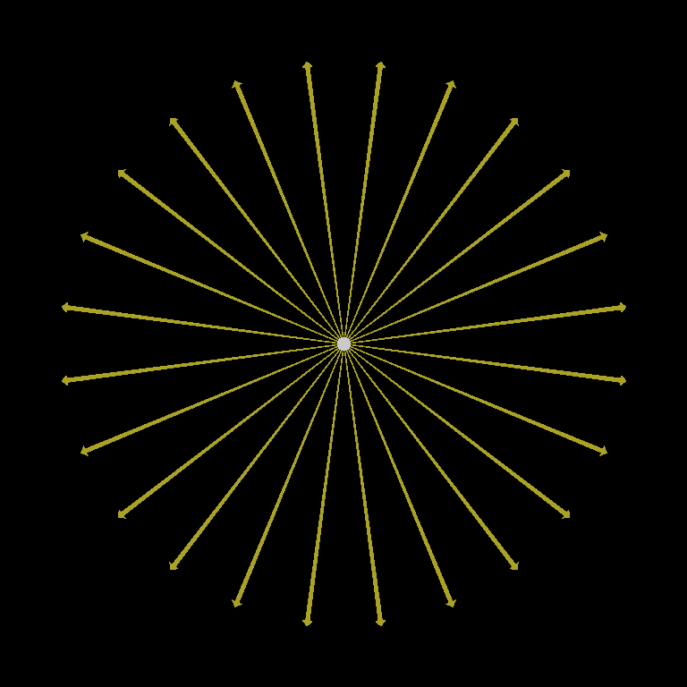
Solving this properly for more than one dimension not only involves multiple variables, and navigating the more involved boundaries of each falloff curve, it also requires testing many gradient direction possibilities. One could try deriving a formula that assumes no restrictions on the directions that gradients can point, however the bound produced by such a formula would likely be quite loose. Noise is typically implemented using a table or generator that only yields a small set of possible vectors.
Numerical Precision
Finally, the process of evaluating a formula this elaborate might incur enough numerical precision loss, that it could not be trusted to accurately reflect the noise’s range. It would be better to directly reproduce promising scenarios in the noise, and search for the value methodically.
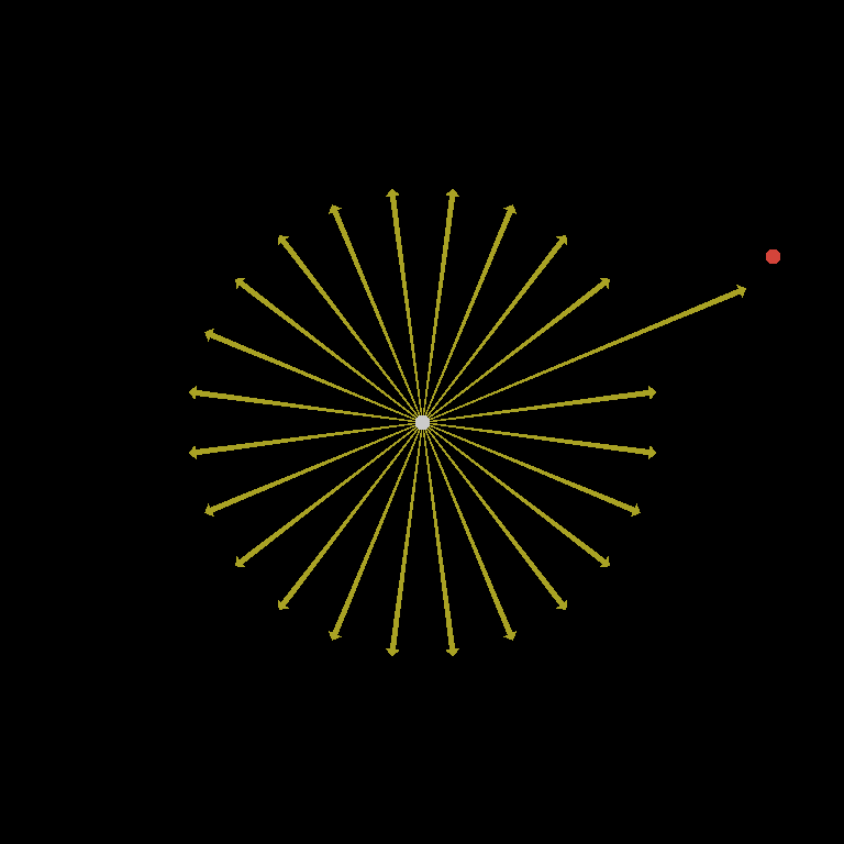
Gradient Ascent… and Gradients
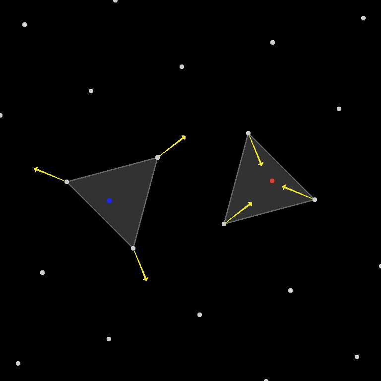
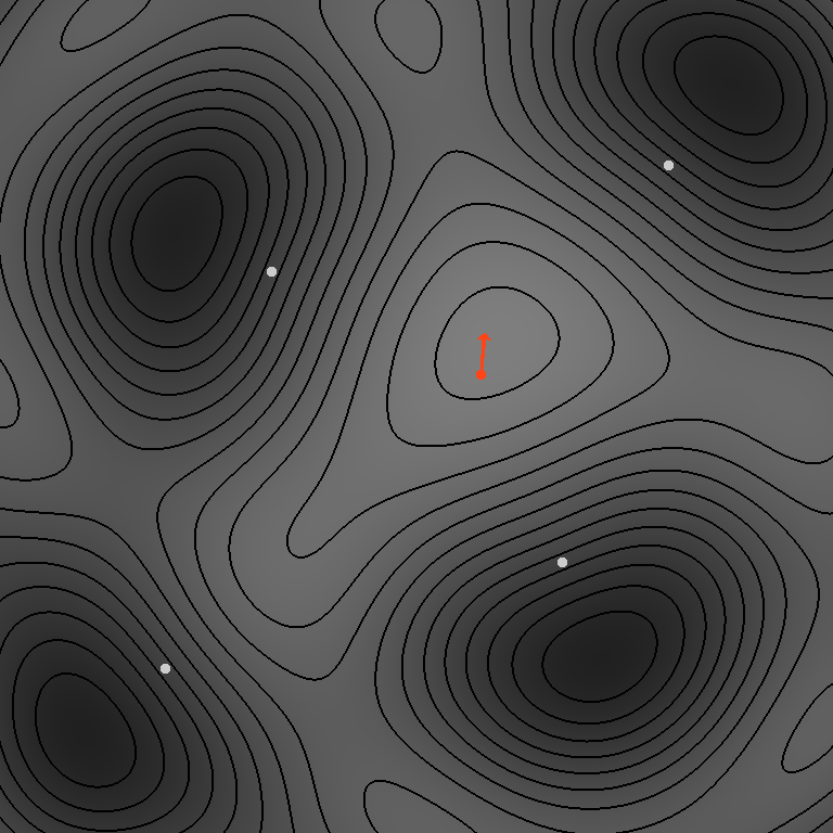
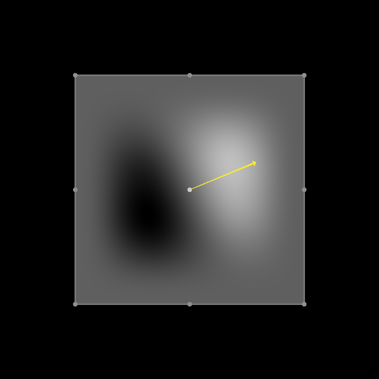
I decided on a Gradient Ascent based technique to better search for the maximizing noise value. Gradient Ascent refers to the process of starting at one point on some function, and repeatedly moving by a small amount in the most-uphill direction until a local maximum is reached. Not to be confused with the gradient vectors chosen at each vertex in the gradient noise, the name of this process refers to the function’s partial derivative vectors (i.e. “gradients”) sampled at each point along the path it takes. It is similar to Gradient Descent, only differing in the direction it moves. As discussed previously, it doesn’t matter whether we find the minimum or the maximum, so this decision is somewhat arbitrary.

Vertex Gradients
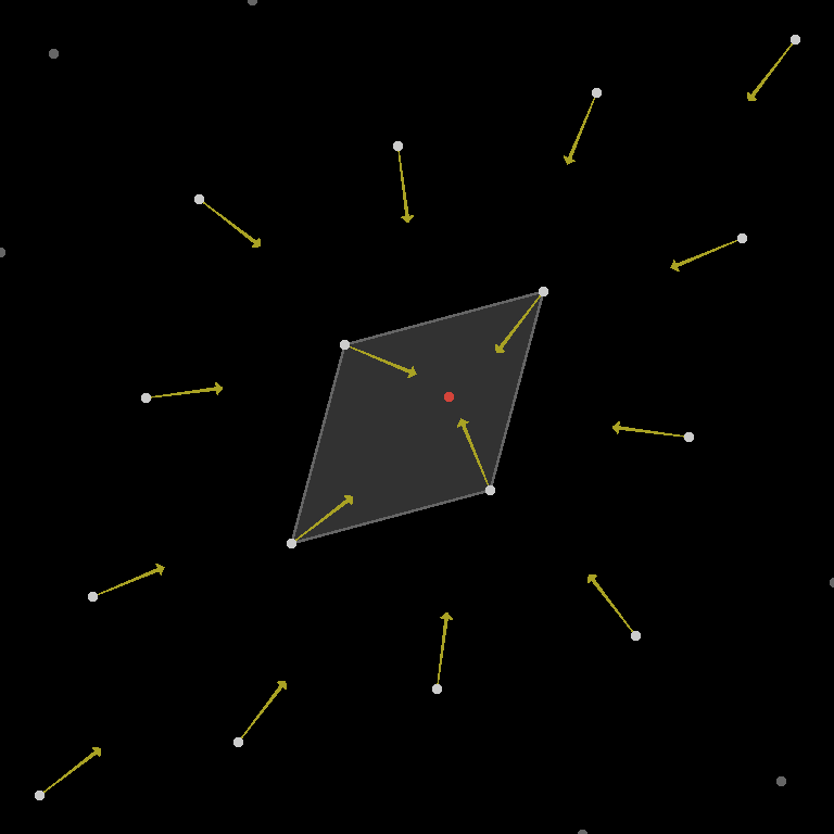
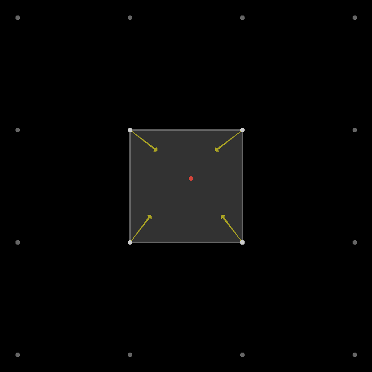
To ensure we can quickly find the global maximum, it is necessary to influence the search to consider vertex gradient configurations that are likely to yield it. To do this, I perform the gradient ascent on a modified noise. Instead of choosing randomized gradient vectors, it repeatedly refreshes the gradients at each nearby vertex, so as to maximize the noise value at the current evaluation point. This starts the search off in a good configuration, and updates it along the way.
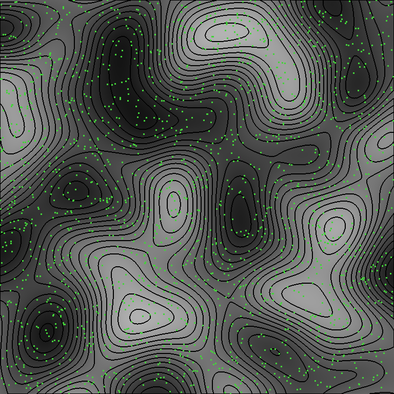
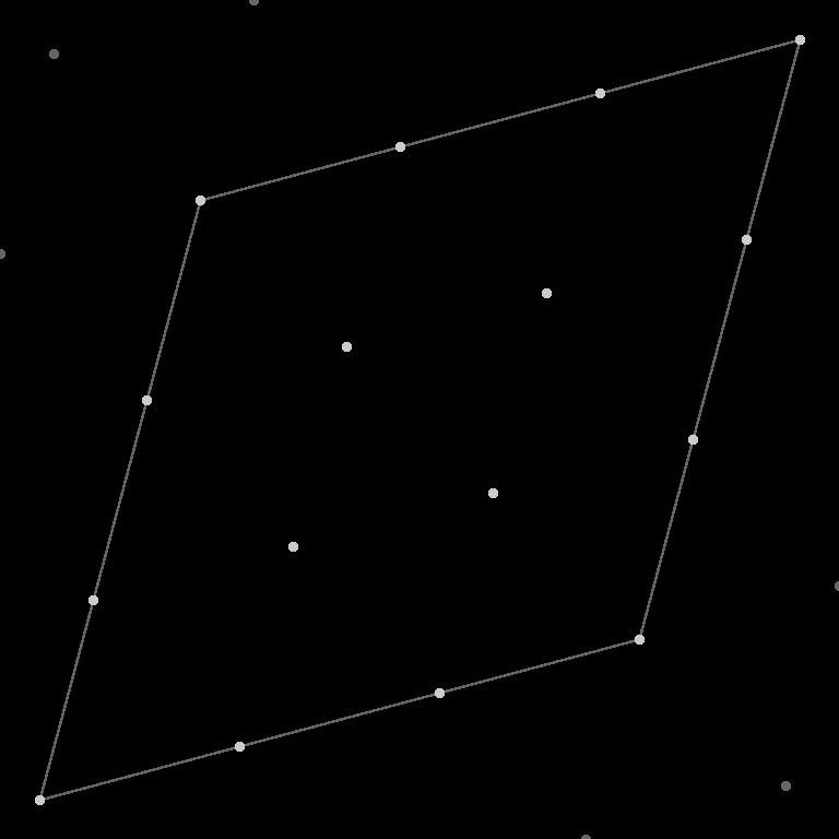
Multiple Starting Locations
Setting the gradients this way eliminates the problem of searching for good configurations. However, it is still important to try multiple starting locations. There are three main reasons not all paths will lead to a global maximum. First, if the starting gradient configuration isn’t yet the ideal case, it is possible to converge on a local maximum before a better configuration is found. Second, it may not be guaranteed that every local maximum will be a global maximum, even with the ideal gradients. Finally, it is possible for numerical precision loss to produce slightly different results in the symmetric cases which should theoretically produce the same value.
Termination
There needs to be a way to stop the ascent once the evaluation point is not able to move any higher. I chose the following solution, which seemed to work well: (1) check if adding the movement vector changed the location of the evaluation point, (2) if not, double the movement and re-try for a few iterations, and (3) stop if it remained stationary. The goal of this is both to avoid irrecoverably overshooting the max and to reach the top of the hill as accurately as possible within the limits of floating point precision.
Starting with Simplex
We can now look at implementing this for various classes of gradient noise. I will start with Simplex/OpenSimplex, because they were my first focus when writing this tool. They also produce good results for a lot of use cases, and it’s clear how to compute their derivatives.

Because Simplex, OpenSimplex2, and 2014 OpenSimplex all use the same contribution falloff function, all that’s needed is a way to place the vertices in the correct layout. This can be accomplished using a for-loop on a small section of the skewed noise coordinates, and transforming each point’s position using the appropriate unskew constant. I chose a 4x4x…x4 grid region which covers all vertices required by any of the noise algorithms. Then, since efficiency isn’t paramount, we can skip the unique grid traversal component of each noise, and simply iterate over every vertex during evaluation. Most vertices will not fall in range of a given evaluation point, but almost all of them are used at some point in at least one noise. It should be noted that OpenSimplex2(F) and original Simplex never consider points outside the central 2x2x…x2 range in this layout. Only OpenSimplex2S and 2014 OpenSimplex do.
For many of the algorithms, the unskew constant can be taken directly from the noise code. But for some, a substitute is required from another noise. OpenSimplex2S 3D and OpenSimplex2(F) 3D+ use a much different grid traversal to Simplex, which consists of multiple offset sub-grids. However, the grids are isomorphic, so it is possible to compute the normalization as if the noise were the original Simplex. Note that the 3D cases require a slightly different constant, which produces a rotated version of the grid to match the gradients. The 4D cases can borrow the constant directly. Someday I will write an article on exactly how the OpenSimplex2 noises work.
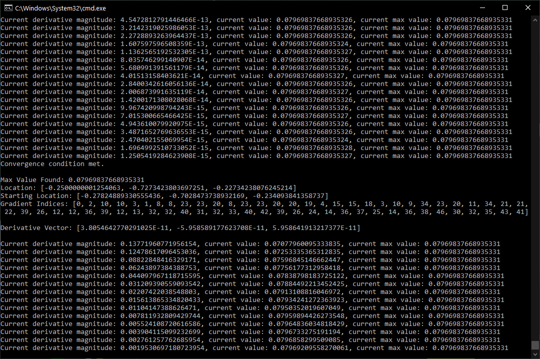
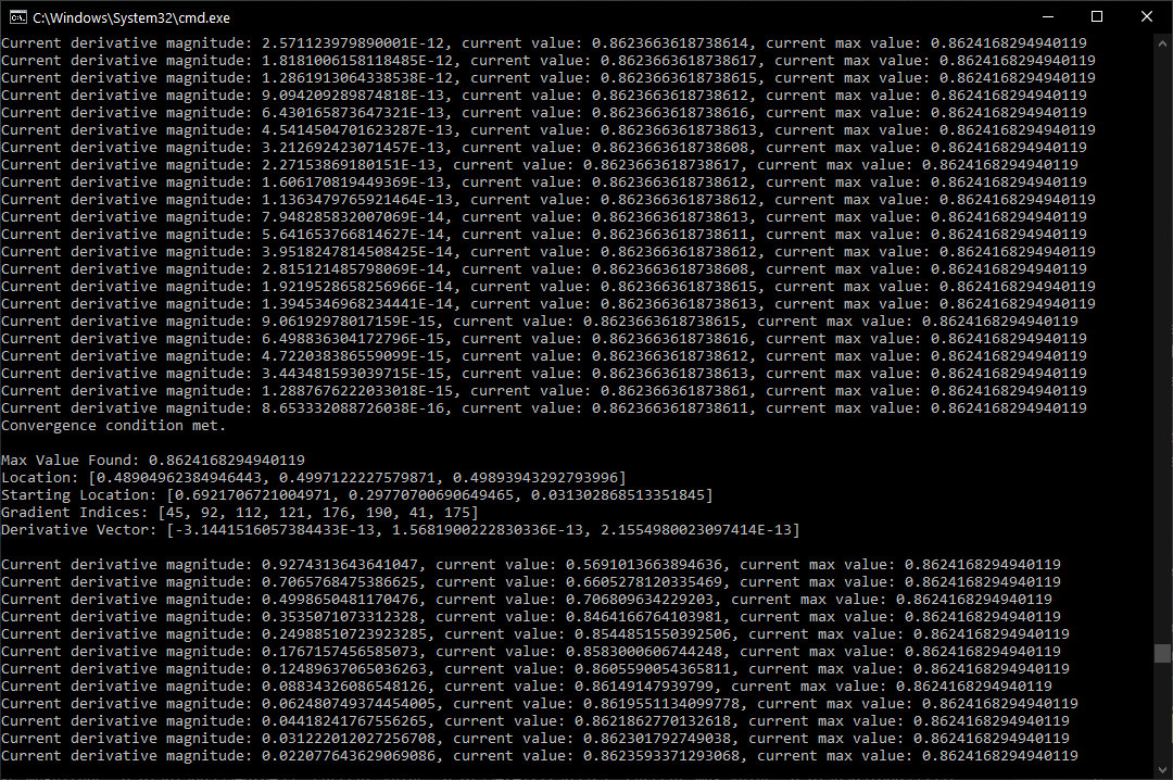
Once the points are in place, we need a loop that repeatedly tries new starting locations for the gradient ascent. At the beginning of this loop, there will be a generator that chooses points inside the target grid location. This will be followed by an internal loop, which performs the gradient ascent process itself. During each iteration of this loop, we will first choose the maximizing gradients for each vertex. That is – the gradients whose ramp value at the evaluation point is the highest. Then, we can compute the value and derivative vector of the noise. The value is used to update the current maximum, while the derivative vector tells us the direction and amount to move in.
Finally, I added a variable to control the rate of movement, as well as the stop condition described previously.
Ye Olde Perlin
Perlin noise is an older gradient noise algorithm. It has problems with directional variety, so I don’t usually recommend it in the absence of mitigation measures such as 3D+ domain rotation. I will elaborate on this more in my next blog post, but for now we can compute its bounds.
Perlin chooses gradient vectors at each vertex, in the same manner as Simplex. It differs, however, in the shape of its grid, and how the gradient ramps are blended. The grid is simply square or cubic, which is easy to port from the Simplex normalizer by removing the unskew step. We also only need to iterate over a 2x2x…x2 region, because there aren’t any common Perlin implementations which consider more than the current grid cell.
The gradient contributions, on the other hand, are combined using linear interpolation smoothed out by a symmetric fade-curve, rather than direct summation. At first glance, this may seem to require significant rewrite. However, the interpolation can actually be decomposed into individual falloff functions, which can be added together in the same way. This is largely because, at the core of each linear interpolation lerp(a, b, t) = (1-t)*a + t*b, both sides are joined by an addition. When the successive interpolations are fed into each other, the effective weight of each vertex only gains more terms: lerp(lerp(a, b, x), lerp(c, d, x), y) = (1-x)*(1-y)*a + (1-x)*y*b + x*(1-y)*c + x*y*d. Plugging in the fade-curves for x,y,… and considering that 1-fadeCurve(t) = fadeCurve(1-t), each vertex’s falloff function can be expressed as fadeCurve(1-|dx|)*fadeCurve(1-|dy|)*.... This leads to a lot of repeated computation, but efficiency isn’t super important here. Using this, we can compute the value and derivative just as we did in the Simplex case.
In some cases, I found that the iteration got hung up when given a more involved gradient set. I discovered this was occurring when the coordinate left the bounds of the grid cell, so I implemented a check to constrain its range. With that in place, all the problematic cases terminated.
Applying the bounds
The most straightforward and reasonably efficient way to apply the result to the noise, is to compute its reciprocal NORMALIZATION_CONSTANT = 1.0 / MAX_VALUE and multiply the noise value by it before it is returned.
public double noise3(double x, double y, double z) {
    ...

    return value * NORMALIZATION_CONSTANT;
}
This works well for noise that does not use gradient tables, or if the gradient tables are shared by many different functions. However, the value can also be baked into the tables directly. For example, { 1, 1, 0 }, { -1, 1, 0 } would become { NORM_CONST, NORM_CONST, 0 }, { -NORM_CONST, NORM_CONST, 0 }, or { 0.130526192220052, 0.99144486137381 } would become { 0.130526192220052 * NORM_CONST, 0.99144486137381 * NORM_CONST }. If your language supports it, you can modify your table using a loop inside a static block or static constructor, instead of applying it manually.
static {
    for (int i = 0; i < GRAD.length; i++) {
        GRAD[i] *= NORMALIZATION_CONSTANT;
    }
}
In some cases, a bound of [0, 1] is desired instead. In this case, the resulting noise value can be multiplied by half the normalization constant, then 0.5 added. If the table solution is desired, then the multiplication can be performed in the table, but the addition must still be performed on the value directly. This makes techniques such as ridged noise and cave tunnels require an extra step to reverse this, but can make other math more intuitive.
Precision Notes
Due to slight precision differences between the normalizer and actual noise implementations, there is still a chance for the result to be slightly off. One hopeful fact is that there is a small amount of leeway regarding a number’s reciprocal. For example, computing 1.0 / 0.0796983766893533 returns 12.547307003476112. But 0.0796983766893533 * 12.547307003476112 actually returns 0.9999999999999999. Interestingly, up to 12.547307003476114 can be used without the result exceeding 1.0 in double precision. I don’t know if this is enough margin to prevent noise values such as 1.0000000000000002 from ever occurring, so someday I might find the time to recreate the maximizing scenarios within the actual noise algorithms. For now, though, this is the most accurate existing solution to this problem that I am aware of.
There is also slightly more opportunity for error when the normalization is applied to the gradient tables, rather than to the result directly. To account for this, I added an optional step which bakes a user-specified normalization constant into the gradient tables before searching for the bounds. This way a user can at least check if their constant passes this test.
Another Article
After writing the majority of this article, I discovered another on the topic. It discusses a similar gradient ascent process, and even goes into an algebraic derivation. From a mathematical perspective, it is very interesting. Critically, however, their approach assumes a continuous range of vertex vector possibilities, so it will not produce a tight bound. The article also focused on Perlin noise, with no mention of its axis bias problems, simplex replacements, or effective mitigation measures. I can only assume that the author’s choice on the matter was influenced by the dense forest of other sources which also focus on this noise. However, sources which portray Perlin noise in this unaddressed manner create ongoing problems in the procedural generation community. Indeed, this will be the focus of my next blog post.
Code & Usage
I’ve updated the code at my github repository to be more organized, and to include implementations for both noise cases. To use them, first set the appropriate constants at the top of the code. For both, you will need to specify the dimensionality of the noise, and provide the gradient array. In each case, there are additional noise-specific parameters. At the top, there is a CONVERGENCE_RATE constant. This can be increased if the normalizer is not making progress fast enough. However, if you make the value too large, the normalizer may lose some accuracy.
private static double CONVERGENCE_RATE = 1.0 / 512;
    // 2D Simplex with 24 gradients
    public static int N_DIMENSIONS = 2;
    public static double UNSKEW_CONSTANT = -0.211324865405187;
    public static double FALLOFF_RADIUS_SQ = 0.5;
    public static double[][] GRADIENTS = new double[][] {
        { 0.130526192220052,  0.99144486137381},
        { 0.38268343236509,   0.923879532511287},
        { 0.608761429008721,  0.793353340291235},
        { 0.793353340291235,  0.608761429008721},
        { 0.923879532511287,  0.38268343236509},
        { 0.99144486137381,   0.130526192220051},
        { 0.99144486137381,  -0.130526192220051},
        { 0.923879532511287, -0.38268343236509},
        { 0.793353340291235, -0.60876142900872},
        { 0.608761429008721, -0.793353340291235},
        { 0.38268343236509,  -0.923879532511287},
        { 0.130526192220052, -0.99144486137381},
        {-0.130526192220052, -0.99144486137381},
        {-0.38268343236509,  -0.923879532511287},
        {-0.608761429008721, -0.793353340291235},
        {-0.793353340291235, -0.608761429008721},
        {-0.923879532511287, -0.38268343236509},
        {-0.99144486137381,  -0.130526192220052},
        {-0.99144486137381,   0.130526192220051},
        {-0.923879532511287,  0.38268343236509},
        {-0.793353340291235,  0.608761429008721},
        {-0.608761429008721,  0.793353340291235},
        {-0.38268343236509,   0.923879532511287},
        {-0.130526192220052,  0.99144486137381}
    };
    // 3D Perlin
    private static int N_DIMENSIONS = 3;
    private static FadeCurveType FADE_CURVE_TYPE = FadeCurveType.Quintic;
    private static double[][] GRADIENTS = new double[][] {
        { 1,  1,  0},
        { 1, -1,  0},
        {-1,  1,  0},
        {-1, -1,  0},
        { 1,  0,  1},
        { 1,  0, -1},
        {-1,  0,  1},
        {-1,  0, -1},
        { 0,  1,  1},
        { 0,  1, -1},
        { 0, -1,  1},
        { 0, -1, -1}
    };
When I first wrote these tools, I used them as practice for Java streams. Indeed, there is a lot of that left in the code, though there are newer parts which I wrote using ordinary loops. Functionally, they serve in-place of for-loops and array initialization. I used them to inline a lot of the vector math. If you aren’t familiar with them, then you may need to research how they work to best understand the code.
    for (int k = 0; k < N_LATTICE_VERTICES; k++) {
        double skew = UNSKEW_CONSTANT * Arrays.stream(latticePointsCubespace[k]).sum();
        latticePoints[k] = Arrays.stream(latticePointsCubespace[k]).mapToDouble(v -> v + skew).toArray();
    }
Console Output